第 7 章 Annotation and Maps
xfun::download_file("https://www.dropbox.com/s/7b3nbgfx5bgft8g/drake_annotationmaps.Rdata?dl=1")
load("drake_annotationmaps.Rdata")
7.1 地圖基本元素
多由point, line, polygon(多邊體)組成。
point: 如景點位置;geom_point
line: 如河流; geom_path
polygon: 如臺北市範圍界線;geom_polygon
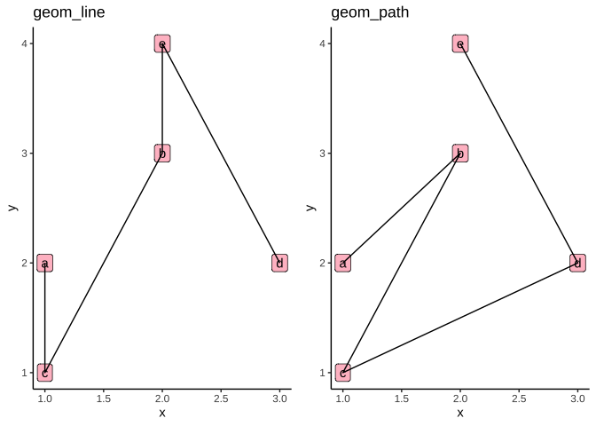
geom_line與geom_path差異在:
geom_line: 以x值排序繪成。
geom_path: 以(x,y)出現順序繪成。
df0 = data.frame(
  x=c(1,2,1,3,2),
  y=c(2,3,1,2,4),
  label=c("a","b","c","d","e")
)
df0 %>%
ggplot(aes(x=x,y=y))+
geom_label(
aes(label=label), fill="pink"
)-> plotbase0
plotbase0list_graphs ={
list_graphs <- list()
plotbase0+geom_line()+labs(title="geom_line") ->
list_graphs$geom_line
plotbase0+geom_path()+labs(title="geom_path") ->
list_graphs$geom_path
list_graphs
}
7.1.1 Point, line, polygon
為方便說明,先創造格線底圖myGrids:
myGrids ={
  ggplot()+theme_linedraw()+
  scale_x_continuous(limits=c(0,6),breaks=0:6,
                     expand=expand_scale(add=c(0,0)))+
  scale_y_continuous(limits=c(0,6),breaks=0:6,
                     expand=expand_scale(mult = c(0,0))) ->
  myGrids

myGrids
}- theme_linedraw(): 圖面每個breaks均有格線
- expand=…: 用來設定在資料limits上限及下限要再延伸多少.
expand_scale(add=c(a1,a2))下限減a1,上限加a2;或expand_scale(mult=c(m1,m2))下限減limits長度m1倍,上限加其m2倍。
7.1.2 Matrix expression
後面介紹到地圖常用的simple features時,因其格式多以矩陣方式輸入,故在此也用矩陣說明。
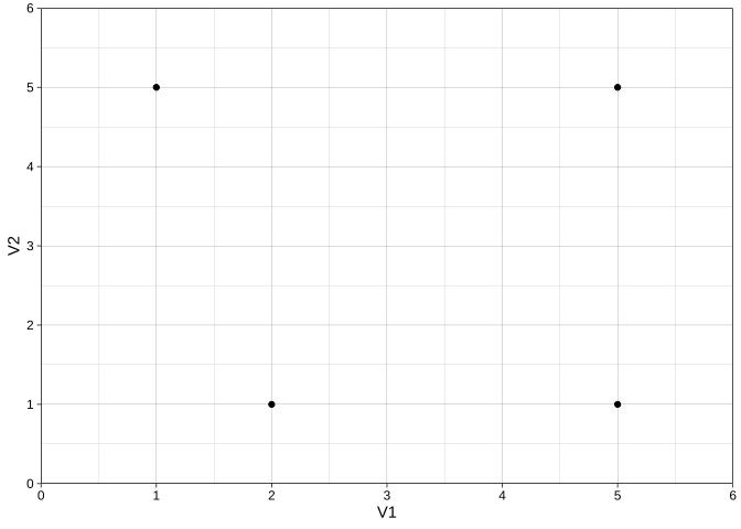
用rbind()產生\(4\times 2\)矩陣,代表在xy平面的三個點:
list_geometryData = new.env()

addPoint = {
  list_geometryData$points <-
    rbind(
      c(1,5),
      c(2,1),
      c(5,1),
      c(5,5))
}

list_geometryData$hole <-
    rbind(
      c(2,4),
      c(3,2),
      c(4,3)
    )

list_geometryData
矩陣as.data.frame後,會形成V1, V2名稱欄位。
list_geometryData$points %>%
  as.data.frame()
myGrids +
geom_point(
data=as.data.frame(list_geometryData$points),
aes(x=V1,y=V2)
) 
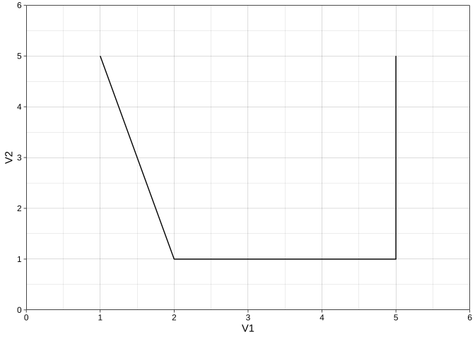
myGrids +
  geom_path(
    data=as.data.frame(list_geometryData$points),
    aes(x=V1,y=V2)
  )
myGrids +
  geom_polygon(
    data=as.data.frame(list_geometryData$points),
    aes(x=V1,y=V2)
  )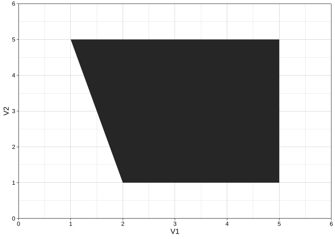
地圖資料中的point, line, polygon便是一系列由:
矩陣
geom
來代表的資訊。
7.1.3 北台灣範例
Exercise 7.1 讀入北台北灣資料:
library(readr)
df_geo_northTW <- read_csv("https://www.dropbox.com/s/6uljw24zkyj7avs/df_geo_northTW.csv?dl=1")
選出COUNTYNAME為“新北市”以geom_polygon繪出如下形狀:
drake$loadTarget$gg_northTW0()
gg_northTW0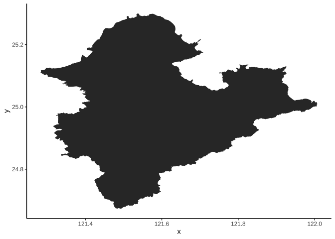
這張圖新北市地圖有什麼問題?
7.1.4 Polygon with holes
polygons = {
  list_graphs$polygon

  list_geometryData$hole <-
    rbind(
      c(2,4),
      c(3,2),
      c(4,3)
    )

  list_graphs$twoPolygons <-
    list_graphs$polygon+
    geom_polygon(
      data=as.data.frame(list_geometryData$hole),
      aes(x=V1,y=V2), fill="white"
    )

}
- 這是假像的解決問題,洞並沒有透出底部格線。
list_geometryData$points %>%
as.data.frame() -> df_part1
list_geometryData$hole %>%
as.data.frame() -> df_part2
df_part1 %>%
mutate(
sub_id=1
) -> df_part1
df_part2 %>%
mutate(
sub_id=2
) -> df_part2
bind_rows(
df_part1,
df_part2
) -> df_all
df_all %>%
mutate(
group_id="A"
) -> df_all
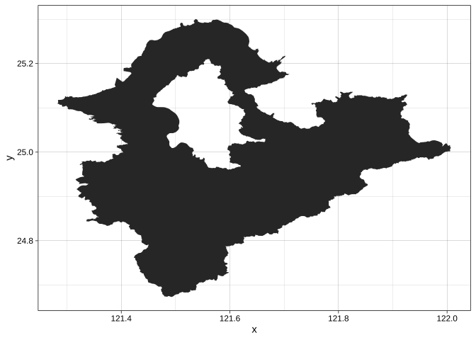
df_allgg_polygonTrue = {
myGrids +
geom_polygon(
data=df_all,
aes(x=V1,y=V2, group=group_id, subgroup=sub_id)
)
}drake$loadTarget$gg_polygonTrue()
gg_polygonTrue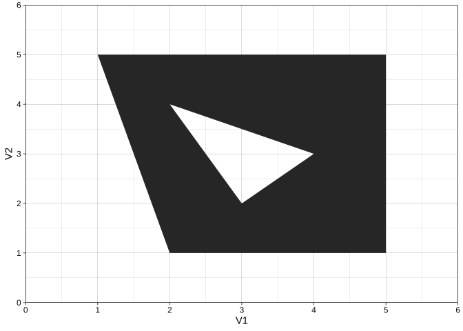
polygonWithHoles = {
  df_all %>%
  add_row(
    V1=c(4,4.5,4.5),
    V2=c(1.5,1.5,2),
    sub_id=c(3,3,3),
    group_id="A"
  ) -> df_all3Subgroups

  myGrids+
    geom_polygon(
      data=df_all3Subgroups,
      aes(
        x=V1,y=V2,group=group_id, subgroup=sub_id
      )
    ) -> polygonWithHoles

polygonWithHoles
}
geom_polygon習慣以subgroup的第一群為含蓋地理區塊,以後的都是holes。但實際應用它會去看誰的polygon邊界在最外圍,最外圍的自然不會是hole,而是outer area。
Exercise 7.2 請繪出如下正確的新北市地形圖。
7.1.5 Multipolygons
使用aes fill用顏色區分polygons
color決定邊界線顏色
polygonWithFillColor = {
  df_geo_northTW %>%
    ggplot()+
    geom_polygon(
      aes(x=x,y=y,fill=COUNTYNAME), color="azure4"
    ) -> list_graphs$northTW
  list_graphs$northTW
}list_graphs$northTWNULL
7.2 Annotation
annotate(geom, x = NULL, y = NULL, xmin = NULL, xmax = NULL,
  ymin = NULL, ymax = NULL, xend = NULL, yend = NULL, ...,
na.rm = FALSE)7.2.1 線、文字
善用:
theme_linedraw(): 來決定座標。
theme_void(): 來得到空白底面。
# load(url("https://www.dropbox.com/s/9n7b1bcs09gnw0r/ggplot_newTaipei.Rda?dl=1")) # 前個練習若沒做出來,執行此行

list_graphs$northTW +
#  theme_linedraw()+
  geom_path(
    data=data.frame(
      x=c(121.55,121.7,121.9),
      y=c(25.1,24.7,24.7)
      ),
    aes(x=x,y=y)
    )+
  annotate(
    "text",
    x=121.9,y=24.71,label="這是臺北市",
    vjust=0
  )+
theme_void()annotate()針對一筆資訊,geom_...()針對多筆資訊使用aes mapping。
7.2.2 圖片
使用annotation_raster():
* 說明: https://ggplot2.tidyverse.org/reference/annotation_raster.html
annotation_raster(raster, xmin, xmax, ymin, ymax, interpolate = FALSE)library(magick)
# download.file("https://mir-s3-cdn-cf.behance.net/project_modules/max_1200/2450df20386177.562ea7d13f396.jpg",
# destfile = "taipei101.jpg")
image_read("https://mir-s3-cdn-cf.behance.net/project_modules/max_1200/2450df20386177.562ea7d13f396.jpg") -> taipei101查看圖片資訊
taipei101 %>%
  image_info() -> taipei101info
# taipei101info

# 檢視圖片高寬比
taipei101info$height/taipei101info$width -> img_asp # image aspect ratio
img_asp
圖片width,height
ggplot()+theme_linedraw()+
  theme(
    panel.background = element_rect(fill="cyan4")
  )

theme_linedraw()+
  theme(
    panel.background = element_rect(fill="cyan4")
  ) -> list_graphs$theme_backgroundCheck

# 圖片底色非透明
taipei101 %>%
  image_ggplot()+
  list_graphs$theme_backgroundCheck
圖片填色(讓背景為透明)
point=“+
image_fill(taipei101, "transparent", point = "+100+100", fuzz = 0) %>% # fuzz=對邊界定義模糊度 %>%
    image_ggplot()+list_graphs$theme_backgroundCheck

image_fill(taipei101,"transparent", point = "+100+100", fuzz=30) %>%
    image_ggplot()+list_graphs$theme_backgroundCheck
轉成raster矩陣資料
image_fill(taipei101,"transparent", point = "+100+100", fuzz=30) ->
  taipei101transparent

taipei101transparent %>%
  as.raster() ->
  raster_taipei101
loc <- c(lon=121.5622782,lat=25.0339687) # Taipei101 經緯度
imgWidth <- 0.13 # Taipei101在圖片佔寬
list_graphs$northTW +
annotation_raster(raster_taipei101,
loc[1]-imgWidth/2,loc[1]+imgWidth/2,
loc[2]-imgWidth/2*img_asp,loc[2]+imgWidth/2*img_asp)調低解析度
image_scale(taipei101transparent,"200") -> taipei101sm
taipei101sm %>% as.raster() -> raster_taipei101sm
list_graphs$northTW +
  annotation_raster(raster_taipei101sm,
                    loc[1]-imgWidth/2,loc[1]+imgWidth/2,
                    loc[2]-imgWidth/2*img_asp,loc[2]+imgWidth/2*img_asp) ->
  list_graphs$northTW2

list_graphs$northTW2
Exercise 7.3 選一張過去展示作品,幫它加上
7.2.3 QR code
library(qrcode)
qrcode_gen("https://bookdown.org/tpemartin/108-1-ntpu-datavisualization/",
           dataOutput=TRUE, plotQRcode=F) -> qr_matrix

qr_dim <- dim(qr_matrix)
qr_matrix %>%
  as.character() %>%
  str_replace_all(
    c("1"="black",
      "0"="white")
  ) -> qr_raster

dim(qr_raster) <- qr_dim

list_graphs$northTW2+
  annotation_raster(qr_raster,121.8,122.0,24.65,24.85)+
  theme_void()
Exercise 7.4 選一張過去展示作品,幫它加上
國立臺北大學logo
QR code, 內容為經濟學系網址: http://www.econ.ntpu.edu.tw/econ/index.php
7.3 Simple features
一種地圖資訊的儲存格式,將地理區域的特徵以點、線、多邊體等簡單幾何特徴記錄。
引入simple feature處理套件
library(sf)7.4 Coordinate Reference Systems (CRS)
包含兩部份:
geographic coordinate reference systems: 經度、緯度,衡量規則通常為WGS84。
projected coordinate reference systems:怎麼把球體上的地理位置投射成2維經緯平面,受投射中心點及投射方法選擇影響。
不同CRS在2維平面投出的地理形狀、兩點距離、兩點角度會有不同結果;在繪圖時需要特別聲明。
CRS設定,2選一:
epsg碼:
proj4string: `+proj=<投射法> A planar CRS defined by a projection, datum, and a set of parameters. In R use the PROJ.4 notation, as that can be readily interpreted without relying on software.
1. Projection: projInfo(type = “proj”) 什麼投射法
2. Datum: projInfo(type = “datum”) 什麼圖資來定義經緯線
3. Ellipsoid: projInfo(type = “ellps”) 什麼橢球體
7.5 讀入shp檔
shp檔其實是由數個檔形成的向量地理圖資,包含:.shp, .shx, .dbf (前三個必需要有)及 .prj等一系列「相同名稱」、「不同副檔名」組成的地理資訊。
sf::read_sf(".shp檔位置")由 https://data.gov.tw/dataset/7442 引入台灣直轄市、縣市界線圖資存在名為dsf_taiwan的物件。
7.6 geom_sf
dsf_taiwan %>%
  ggplot() +
  geom_sf()
7.6.1 常見圖資運算
7.6.1.1 幾何簡化: rmapshaper::ms_simplify()
dsf_taiwan %>%
  rmapshaper::ms_simplify() -> dsf_taiwan_simplify
dsf_taiwan_simplify %>%
ggplot()+geom_sf()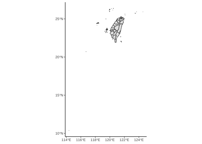
7.6.1.2 切出部份範圍: st_crop()
dsf_taiwan_simplify %>%
  st_crop(c(xmin=119,xmax=122,ymin=22,ymax=25.8)) -> dsf_taiwanCropped
dsf_taiwanCropped %>%
ggplot()+geom_sf()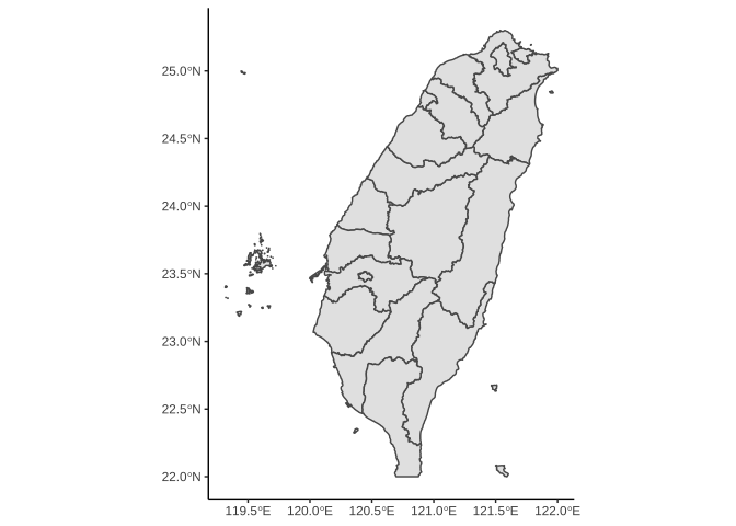
dsf_taiwanCropped %>%
  filter(
    stringr::str_detect(COUNTYNAME, "宜|北|基")
  ) %>%
  ggplot() +
  geom_sf()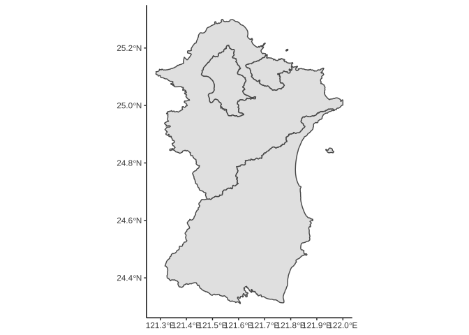
dsf_taiwanCropped %>%
  filter(
    stringr::str_detect(COUNTYNAME, "宜|北|基")
  ) %>%
  ggplot() +
  geom_sf(
    fill="#e3fdfd",
    color="#71c9ce"
  )+
  theme_void()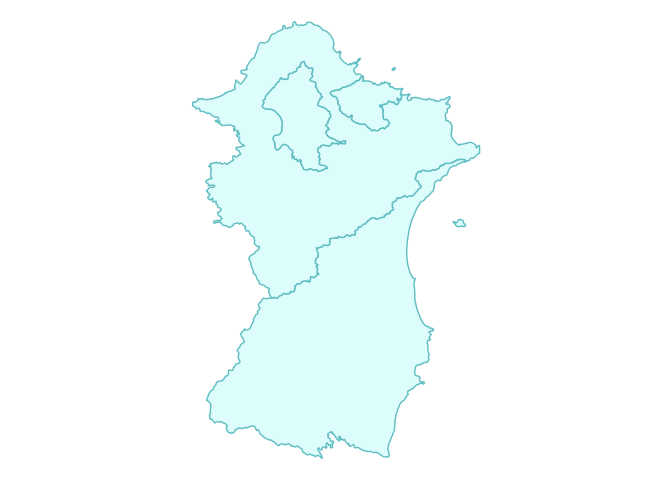
dsf_taiwanCropped %>%
  filter(
    stringr::str_detect(COUNTYNAME, "宜|北|基")
  ) %>%
  ggplot() +
  geom_sf(
    aes(fill=COUNTYNAME),
    color="white", size=0.2
  )+
  colorspace::scale_fill_discrete_qualitative(
    name="縣市"
  )+
  theme_void()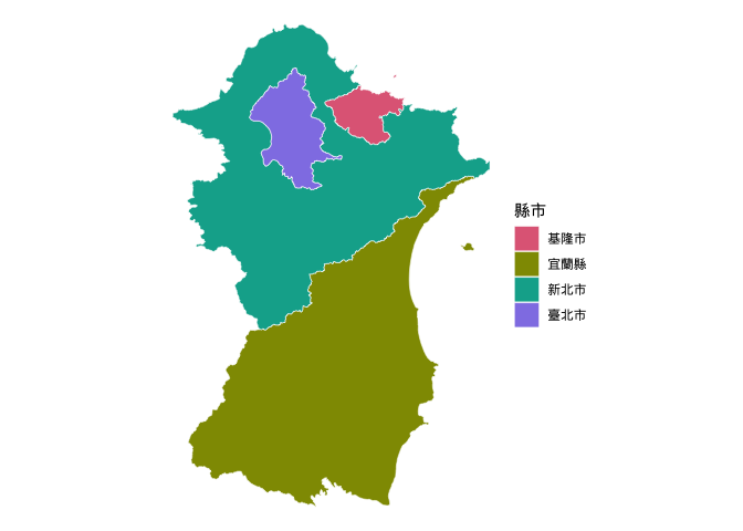
7.7 Open Street Map (OSM)
Online street map consists of:
Bounding Box (bbox): latitudes and longtitudes that crop out the area of geographic data user request.
Features: the features on the map users are interested in. For example, administrative boundaries, parks, buildings, etc. (https://wiki.openstreetmap.org/wiki/Map_Features)
7.7.1 BBox
Use one of the following:
osmdata::getbb(place_name)
osmdata::getbb("new taipei") -> newTaipeiBBox
newTaipeiBBox- https://openstreetmap.org click Export. MUST specify as
c(xmin, ymin, xmax, ymax) # order has to be the samenewTaipeiBBox <- c(xmin=121.28263, ymin=24.67316, xmax=122.00640, ymax=25.29974)7.7.2 Features
- find target feature key and value: https://wiki.openstreetmap.org/wiki/Map_Features
Check available key of features
stringr::str_subset(osmdata::available_features(), "boundary|admin")Use Open Pass Query (
opq(bbox)) to initiate feature query.add_osm_feature(key, value)to add layers of feature of request.Finally,
osmdata_sf()to export data as a simple feature data.
osmdata::getbb("new taipei") -> newTaipeiBBox
dsf_newTaipei <- opq(newTaipeiBBox) %>%
     add_osm_feature(key="admin_level", value="5") %>%
osmdata::osmdata_sf()- OSM returned-features cover different geometries. Each geometry is a separate simple feature dataframe. Collective as a list is what the returned value is, such as dsf_newTaipei. To proceed for graphing, user needs to select the geometry target, such as:
dsf_newTaipei$osm_lines
dsf_newTaipei$osm_multipolygons
Only the extracted geometry element itself is a proper simple feature data frame that is ready for graphing.
dsf_newTaipei$osm_lines %>%
  ggplot()+geom_sf()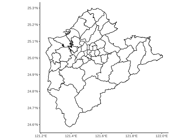
osm_geom_rename
osm資料對於每一個feature的geometry元素皆有命名,且此名稱是所有geometry feature代碼的串接,因此有時名稱會太長超過R內定可容忍長度,而產生如下Error:
dsf_newTaipei$osm_multipolygons %>%
  ggplot()+
  geom_sf()
Error in do.call(rbind, x) : variable names are limited to 10000 bytes
寫成函數方便未來反覆使用
osm_geom_rename <- function(sf_object){
  sf_object %>%
    st_geometry() -> sfc_sf_object
  for(i in seq_along(sfc_sf_object)){
    names(sfc_sf_object[[i]][[1]]) <-
      1:length(names(sfc_sf_object[[i]][[1]]))
  }

  sf_object %>%
    st_set_geometry(
      sfc_sf_object
    ) -> sf_object2
  return(sf_object2)
}
老師將上述函數放在以下網址,同學也可以在setup裡增加以下指令:
xfun::download_file("https://www.dropbox.com/s/8ndtvzqbdb4cb93/data_visulaization_pk.R?dl=1")
source("data_visulaization_pk.R", encoding = "UTF-8")這樣osm_geom_rename()就進來了。
dsf_newTaipei$osm_multipolygons %>%
  osm_geom_rename() %>% # 多插這一行
  ggplot()+
  geom_sf(
    aes(fill=name),
    color="white", size=0.2
  )+
  colorspace::scale_fill_discrete_qualitative()+
  theme_void()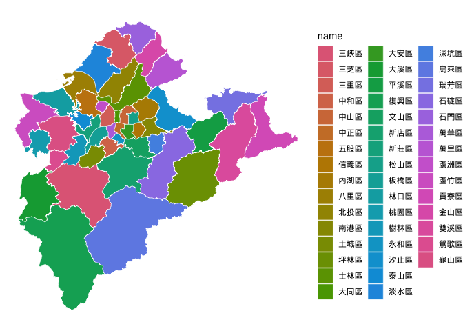
7.8 Google Map
library(ggmap)- define bbox as
newTaipeiBBox2 <- c(left = 121.3, bottom = 24.7, right = 122, top = 25.3)get_map(bbox)to download map data (as a raster); then useggmap()to create a ggplot object.
get_map(newTaipeiBBox2) -> raster_newTaipeiggmap(raster_newTaipei)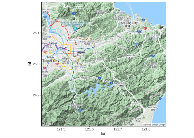
maptype: “terrain”
other maptypes (needs to be set at the
get_map()stage): “terrain,” “terrain-background,” “satellite,” “roadmap,” “hybrid,” “toner,” “watercolor,” “terrain-labels,” “terrain-lines,” “toner-2010,” “toner-2011,” “toner-background,” “toner-hybrid,” “toner-labels,” “toner-lines,” “toner-lite.”
get_map(newTaipeiBBox2, maptype = "toner") -> raster_newTaipeiTonerggmap(raster_newTaipeiToner)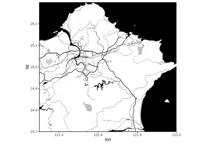
7.8.1 Overlay with geom_sf
ggmap_newTaipei+
  geom_sf(
    data=dsf_newTaipei$osm_multipolygons %>% osm_geom_rename,
    inherit.aes = FALSE,
    alpha=0.3, fill="aliceblue"
  )+
  theme_void() -> ggmap_osm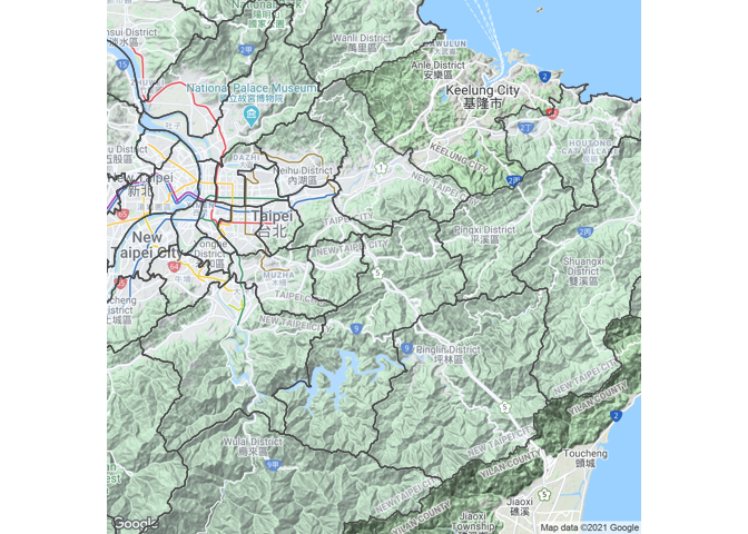
geom_sf has to set inherit.aes=FALSE; otherwise, it will inherit preceeding aes mapping that does not work on sf geom layer.
7.9 2020總統大選面量圖
7.9.1 面量圖(Choropleth Map)
election2020 = jsonlite::fromJSON(
  "https://www.dropbox.com/s/a3torx0p41hheb6/presidentElection2020.json?dl=1"
)
Change column names:
names(election2020) %>%
  stringr::str_which("\\(1|2|3\\)") %>%
  {
    names(election2020)[.] <- c("np", "kmt", "dpp")
    election2020
  } -> election2020_rename
Merge with New Taipei simple feature data:
dsf_newTaipei$osm_multipolygons %>%
  osm_geom_rename() -> dsf_newTaipei2

dsf_newTaipei2 %>%
  left_join(
    election2020_rename %>%
      select(dpp, "鄉(鎮、市、區)別"),
    by=c("name"="鄉(鎮、市、區)別")
  ) -> dsf_newTaipeiDPP
Preliminary plot:
dsf_newTaipeiDPP %>% na.omit() %>%
  ggplot() +
  geom_sf(aes(fill=dpp), color="white", size=0.2) -> ggsf_election2020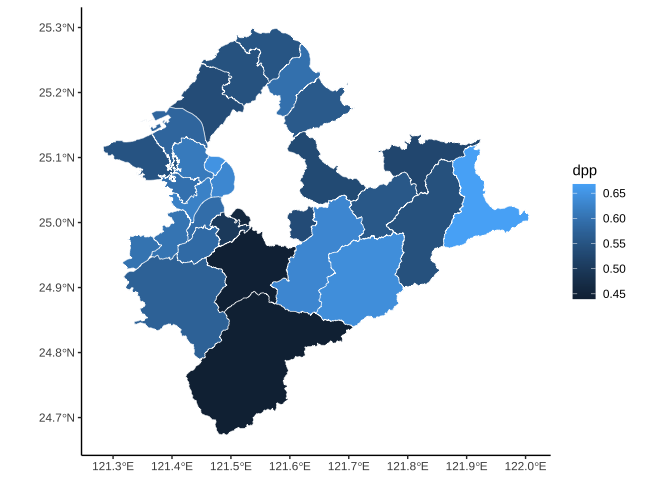
7.9.2 Overlay other map
newTaipei_tonerlite <- get_map(newTaipeiBBox2, maptype="toner-lite")ggmap_newTaipeiTonerLite <- ggmap(newTaipei_tonerlite)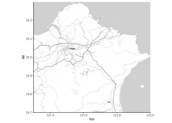
ggmap_newTaipeiTonerLite +
  geom_sf(
    data=dsf_newTaipeiDPP %>% na.omit(),
    mapping=aes(fill=dpp), color="white", size=0.2, alpha=0.7,
    inherit.aes = FALSE # make sure this setup
  ) +
  theme_void() -> ggmap_election2020_1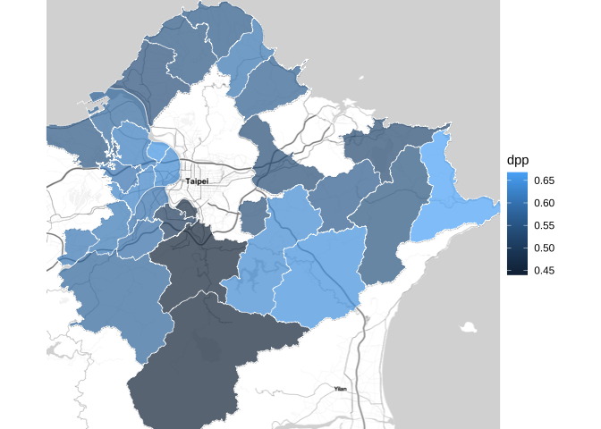
7.9.3 面量圖Refinement
Rescale Data
electionData0 <-
  # drake$loadTarget$dsf_newTaipei()
  # drake$loadTarget$election2020_rename()
  dsf_newTaipei$osm_multipolygons %>%
    osm_geom_rename() %>%
    left_join(
      election2020_rename,
      by=c("name"="鄉(鎮、市、區)別")
    ) %>%
    na.omit()
Diverging sequential by default defines bipolar at the values of -1 and 1. Therefore, we can properly creates bipolar in our data by rescaling data range into [-1, 1].
dppRange = round(range(electionData0$dpp),1)drake$loadTarget$dppRange()list(
fromRange = c(1-dppRange[[2]], dppRange[[2]]),
toRange = c(-1,1)) -> list_rangeselectionData0 %>%
mutate(
dpp_rescaled=
scales::rescale(
electionData0$dpp,
from=list_ranges$fromRange,
to=list_ranges$toRange)
) -> electionDataDesign Scale
colorspace::diverging_hcl(n = 12, h = c(247, 120), c = 100, l = c(30, 90), power = 1.5, register = "kmt_dpp")scale_election = {
breaksPal = seq(
from=list_ranges$toRange[[1]],
to=list_ranges$toRange[[2]],
length.out=5
)
labelsPal = seq(
from=list_ranges$fromRange[[1]],
to=list_ranges$fromRange[[2]],
length.out=5
)
colorspace::scale_fill_continuous_diverging(
palette="kmt_dpp") -> scale_fill_election
scale_fill_election$breaks = breaksPal
scale_fill_election$labels = labelsPal
scale_fill_election$name = "民進黨得票率"
scale_fill_election
}Assemble ggplot
ggsf_election <- {
  ggplot()+
    geom_sf(
      data=electionData,
      mapping=aes(fill=dpp_rescaled), size=0.2, color="white",
      inherit.aes = FALSE
    )+
    scale_election+
    theme_void()
}
gg_electionComplete <-
ggmap_newTaipeiTonerLite +
geom_sf(
data = electionData,
mapping = aes(fill = dpp_rescaled), size = 0.2, color = "white", alpha=0.7,
inherit.aes = FALSE
) +
scale_election +
theme_void()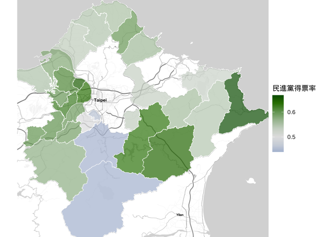
7.10 架構sf data frame
- simple features geometry (for each county)
- simple features column (for all counties)
- set simple features column as a column in a data frame
7.10.1 Geometry (sfg)
主要由以下幾種geometries構成:
POINT, LINESTRING, POLYGON, MULTIPOINT, MULTILINESTRING, MULTIPOLYGON and GEOMETRYCOLLECTION
定義函數均為st_<geometry type>(<geometry record>):
一點:st_point
point <- st_point(
  c(2,3)
)
point %>% ggplot()+geom_sf()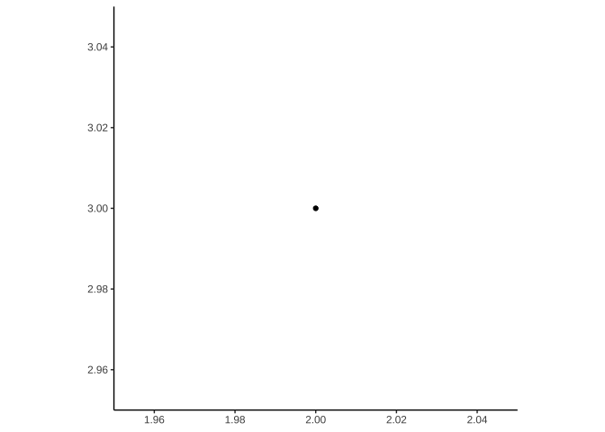
數個點:st_multipoint
mpoint <- st_multipoint(
    rbind(c(1,0),
        c(2,3),
        c(-1,2))
)
mpoint %>% ggplot()+geom_sf()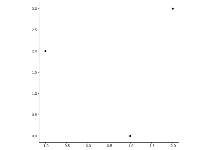
一條線:st_linestring
line <- st_linestring(
    rbind(c(1,0),
        c(2,3),
        c(-1,2))
)
line %>% ggplot()+geom_sf()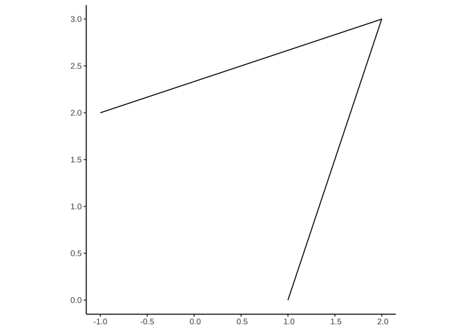
數條線: st_multilinestring
mline <- st_multilinestring(
  list(
    rbind(
      c(1,0),
      c(2,3),
      c(-1,3)),
    rbind(
      c(-2,3),
      c(-1,-1))
    )
  )
mline %>% ggplot()+geom_sf()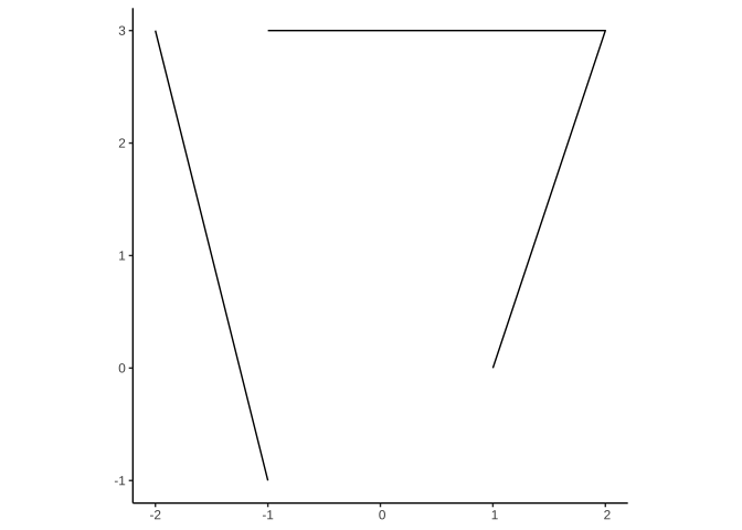
一個多邊體:st_polygon
outer = {
  rbind( # 外圍
    c(1,5),
    c(2,1),
    c(5,1),
    c(5,5),
    c(1,5)) # 必需自行輸入起點close it
}
hole = {
rbind( # 洞
c(2,4),
c(3,2),
c(4,3),
c(2,4)) # 必需自行輸入起點close it
}poly <- st_polygon(
list(
outer,
hole
)
)poly %>% ggplot()+geom_sf()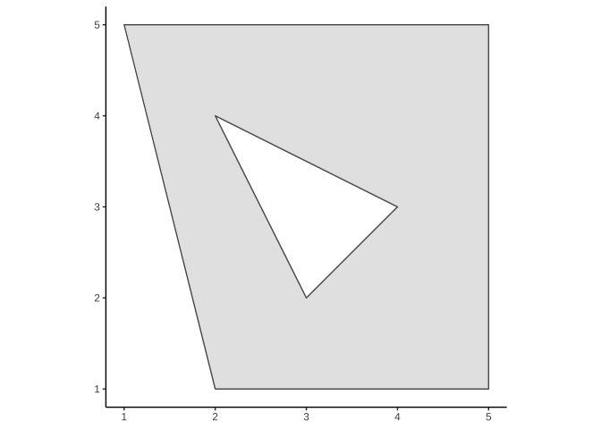
sf::st_polygon(sf)與ggplot2::geom_polygon(ggplot2)對多邊體格式定義差異:
sf下多邊體的最後一個座標必需是第一個座標;ggplot2則不用,自動假設連回第一個 。
sf以第一個ring(即多邊體邊界一圈)為outer ring,其餘為holes。ggplot2則需定義group及subgroup兩個變數後,才能自動判斷哪個ring為ourter,哪個ring為holes。
數個多邊體:st_multipolygon
outer2 <- outer + 12
hole2 <- hole + 12

mpoly <- st_multipolygon(
  list(
    list(
      outer,
      hole
    ),
    list(
      outer2,
      hole2
    )
  )
)
mpoly %>% ggplot()+geom_sf()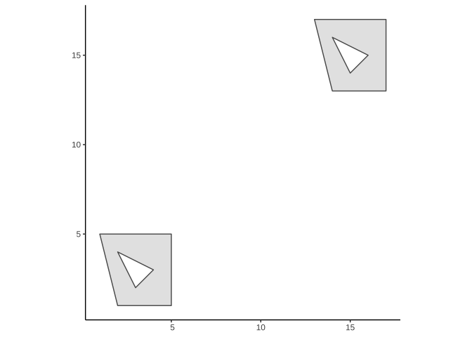
複合幾何收藏:st_geometrycollection
sf::st_geometrycollection(
  list(
    point, mpoint,
    line, mline,
    poly, mpoly
  )
) %>% ggplot()+ geom_sf()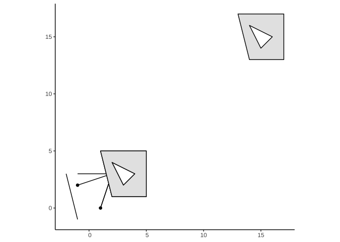
7.10.2 Column (sfc)
建立geometry欄位
st_sfc() to form simple features column.
sfg_county1 <- st_polygon(list(
  outer,hole
))
sfg_county2 <- st_polygon(list(
  outer2, hole2
))

sfc_county12column <- st_sfc(sfg_county1,sfg_county2)

sfc_county12column %>% ggplot+geom_sf()
設定CRS
架構sfc後,最好也順便設定CRS:
sfc_county12column %>%
  st_set_crs(4326) -> # EPSG: 4326
  sfc_county12column
7.10.3 與data frame合併 (sf)
形成sf object: a data frame with a geometry column
Given a data frame, say df, we can attach a geometry column (sfc), say geo_column, through:
st_set_geometry(df,geo_column)df_county12 <- data.frame(
name=c("county1","county2"),
population=c(100,107)
)
df_county12 %>%
st_set_geometry(sfc_county12column) -> df_county12
df_county12 %>% names7.10.4 儲存成shp檔
dir.create("county12")
write_sf(df_county12,"county12/county12.shp")
當然如果只是個人要用,或確信對方也使用R,你也可以存成Rda檔。
save(df_county12,file="df_county12.Rda")之後再:
load("df_county12.Rda")Exercise 7.5 資料來源:政府資料開放平台(https://data.gov.tw/dataset/73233)
執行取得sf_mrt_tpe
load(url("https://www.dropbox.com/s/uvco1te2kbs6o01/MRT_Taipei.Rda?dl=1"))其中代號’O’為「中和新蘆線」、’BL’為「板南線」,只取出此兩線,並形成一個sf data frame含有以下欄位:
路線名稱
geometry: 代表各路線的「點、線」圖。
7.11 更多其他圖資運算
7.11.1 CRS轉換: st_transform()
# 取出spData套件附的world data
data(world,package="spData")
class(world) # 已是sf object

# 目前CRS
world %>% st_crs

world %>% st_geometry() %>%
  ggplot()+geom_sf()
更換CRS
world %>%
  st_transform(crs="+proj=laea +y_0=0 +lon_0=155 +lat_0=-90 +ellps=WGS84 +no_defs") -> world_proj

world_proj %>%
  ggplot()+geom_sf()
7.11.2 找中心點: st_centroid()
找polygon中心點
形成新的sf object,有相同data frame但geometry column只是中心點的point geometry.
如果一筆feature資料有多個中心點,可以設定:
st_centroid(..., of_largest_polygon = T)
load(url("https://www.dropbox.com/s/elnvocol0nnkcc9/sf_northTaiwan.Rda?dl=1"))sf_northTaiwan %>%
st_centroid(of_largest_polygon = T) ->
sf_centroid_northTaiwan
sf_centroid_northTaiwan7.11.3 輸出座標: st_coordinates()
找中心點有時是為了做圖加上新的geom_point layer,還會再進行geom_point layer data frame架構:
sf_centroid_northTaiwan %>%
  st_coordinates() -> coord_centroid_northTaiwan # 取出座標

coord_centroid_northTaiwan

sf_northTaiwan$x_centroid <- coord_centroid_northTaiwan[,"X"]
sf_northTaiwan$y_centroid <- coord_centroid_northTaiwan[,"Y"]
sf_northTaiwan %>%
ggplot()+
geom_sf()+
geom_point(
aes(
x=x_centroid,y=y_centroid,
shape=COUNTYNAME, color=COUNTYNAME
), size=2
)