第 6 章 Map
mp <- econDV2::Map()6.1 Geographic geoms
6.1.1 Point, Line and Polygon
ggplot2 is equipped with geoms that can draw all kinds of geographic structure.
fourPoints <- data.frame(
    x=c(2, 3, 5, 3),
    y=c(-1, 0, 6, 6)
)
geometry <- list()
geometry$ggplot <- function(){
  ggplot(
    data=fourPoints,
    mapping=aes(
      x=x, y=y
    )
  )
}
Points:
geometry$points <- geometry$ggplot() + geom_point()
geometry$points
Path:
geometry$path <- geometry$ggplot() + geom_path()
geometry$path
Polygon
geometry$polygon <- geometry$ggplot() + geom_polygon()
geometry$polygon
6.1.2 Multipolygons
- A school consists of many buildings
bigArea <- data.frame(
  order=1:7,
  x=c(1, 5.5, 5.5, 1,
    7, 8, 9),
  y=c(-2, -2, 7, 7,
    8, 8 , 2),
  building=c(rep("building1", 4), rep("building2", 3)), # same school
  contour=c(rep("outer",4), rep("outer",3)) # two different buildings
)

# draw each building separately
ggplot()+geom_polygon(
  data=bigArea,
  mapping=aes(x=x, y=y, group=building)
)geom_polygoncan draw a polygon with hole(s) by usinggroupandsubgroupaesthetics, with hole(s) as a polygon inside another.- A building with a courtyard has two contours (one for the outer contour, the other for the courtyard contour). Both contours are polygons belong to the same group, but different subgroups.
fourPoints$building="building1"
fourPoints$contour="courtyard"
fourPoints$order=8:11
bigArea |> names()
bigAreaWithHoles <-
  dplyr::bind_rows(
    bigArea,
    fourPoints
  ) |> arrange(building, order)

View(bigAreaWithHoles)

ggplot(
  data=bigAreaWithHoles
) +
  geom_polygon(
    aes(
      x=x, y=y,
      group=building,
      subgroup=contour
    )
  )
6.1.3 Fill polygons
- You can give different polygons different fills.
ggplot(
  data=bigAreaWithHoles
) +
  geom_polygon(
    aes(
      x=x, y=y,
      group=building,
      subgroup=contour,
      fill=building
    )
  )
6.1.4 Application to world map
We apply those geoms to draw some maps.
world = ggplot2::map_data("world")groupcolumn is forgroupaesthetics for polygon.
world0 <- function(color="black", fill="white", size=0.35) {
  ggplot() + geom_polygon(
    data=world,
    aes(
      x=long, y=lat,
      group=group
    ),
  color=color, fill=fill, size=size
  )
}
# Cartesian crs
world0()
# Cartesian with fixed aspect ratio
world0() + coord_fixed()
# Mercator projection: fixed asp, correct direction
world0() + coord_map()
# Mercator projection: fixed asp, correct direction, expand xlim
world0() + coord_map(xlim = c(-180,180))6.2 Choropleth map
- A map with different fills to show certain social-economic data variation.
6.2.1 Backgroup fill and borders
Though ggplot2 has geom function to work on Choropleth graph directly, I recommend to lay out a background map first.
Map data
world = ggplot2::map_data("world")Backgroup map base on Economist style:
world0_background <- function(){
  world0(
    color="white",
    fill="#c8c5be",
    size=0.15)
}world0_background()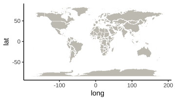
6.2.2 Choropleth layer: value layer
Another layer of geom_polygons but with different fills setup based on social-economic data. Instead of using geom_polygon as the background layer does, geom_map is an easier to use geom for Choropleth graph.
geom_mapis a wrapper ofgeom_polygonbut with a much easier setup for Choropleth map purpose.use
geom_map()+expand_limits()
geom_map(
  data=`social-economic data`,
  mapping = aes(
    map_id = ...,
    fill = ...
  ),
  map =`map data`
)+
expand_limits(
  x=`map data`$long, y=`map data`$lat
)
map datafromggplot2::map_data(can be filtered if needed)social-economic data: a data frame with a column formap_idand a column forfill.map_idcolumn must consist of the levels ofmap data’s region column.fillcolumn: the social-economic data to show.
expand_limitsto ensure that no boundary points are right on the border of the plot.
6.2.2.1 WDI example
Social-economic data
se_data <- jsonlite::fromJSON(
  "https://www.dropbox.com/s/78jr6g6xtjz453b/women_in_parliament.json?dl=1"
)
# View(se_data)ggplot()+geom_map(
data=se_data,
mapping=aes(
map_id=country,
fill=women_in_parliament
),
map=world
)+
expand_limits(x=world$long, y=world$lat)
# geom_map only plot those in the social-economic data
ggplot()+geom_map(
    data=se_data[1:30,],
    mapping=aes(
      map_id=country,
      fill=women_in_parliament
    ),
    map=world
  )+
  expand_limits(x=world$long, y=world$lat)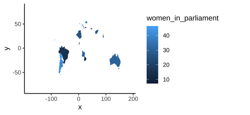
World background ensure every country is on the map.
world0_background() +
  geom_map(
    data=se_data[1:30, ],
    mapping=aes(
      map_id=country,
      fill=women_in_parliament
    ),
    map=world
  )+
  expand_limits(x=world$long, y=world$lat)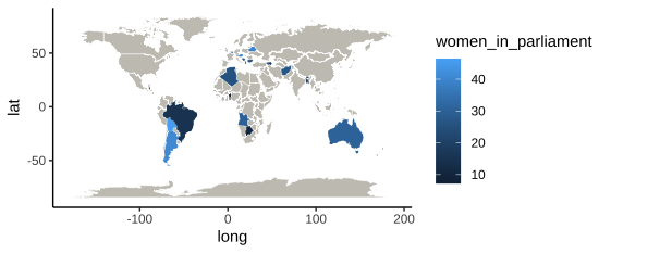
Fixed country name inconsistency between se_data and world data.
se_data |>
  mp$choropleth$rename_valueData_countryname(
  countryColumnName = "country",
  pattern = c(
    "Russia"="Russian Federation",
    "USA"="United States",
    "Iran"="Iran, Islamic Rep.",
    "Egypt"="Egypt, Arab Rep.",
    "Syria"="Syrian Arab Republic",
    "Yemen"="Yemen, Rep.",
    "UK"="United Kingdom",
    "Democratic Republic of the Congo"="Congo, Dem. Rep.",
    "Republic of Congo"="Congo, Rep.",
    "Ivory Coast"="Cote d'Ivoire",
    "Venezuela"="Venezuela, RB"
    )
  ) -> se_data

world0_background() +
  geom_map(
    data=se_data,
    mapping=aes(
      map_id=country,
      fill=women_in_parliament
    ),
    map=world
  )+
  expand_limits(x=world$long, y=world$lat)
choropleth0 <- function(){
world0_background() +
geom_map(
data=se_data,
mapping=aes(
map_id=country,
fill=women_in_parliament
),
map=world
)+
expand_limits(x=world$long, y=world$lat)
}
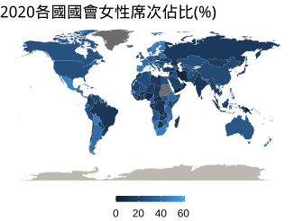
choropleth0() +
theme_void() +
labs(
title="2020各國國會女性席次佔比(%)"
) +
theme(
legend.position = "bottom"
) +
guides(
fill=guide_colorbar(
title=NULL,
barwidth = 4, #input$barwidth
barheight = 0.35, #input$barheight
)
)
# can also
choropleth0() +
scale_fill_gradient(
guide = guide_colorbar(...)
)
6.2.3 Fill colors
6.2.3.1 scale_fill and palette function
scale_fill_continuous(...)by default is based on:
scale_fill_gradient(...) # which is based on the palette function palette_continuous generated by scales::seq_gradient_pal
palette_continuous <- scales::seq_gradient_pal(
  low = "#132B43", high = "#56B1F7"
)- two pigments “#132B43,” “#56B1F7”
palette_continuous(seq(0, 1, by=0.2)) |>
  scales::show_col()
aes(fill=z) will rescale z according to
# for sequential
scales::rescale(z, from=range(z), to=c(0,1))
# for divergin
scales::rescale(z, from=mid.point.value_stretching, to=c(-1,1))scale_fill_discrete(...)by default is based on:
scale_fill_hue(...) # which is based on the palette function palette_discrete generated by scales::hue_pal
palette_discrete <-
scales::hue_pal(h = c(0, 360) + 15, c = 100, l = 65, h.start = 0, direction = 1)- pigments: a hue (色像環)
palette_discrete(3) |> scales::show_col()
palette_discrete(6) |> scales::show_col()DiagrammeR::mermaid("
graph LR
A[continuous palette function]-->B[continuous scales_fill]
C[discrete palette function]-->D[discrete scales_fill]
")6.2.3.2 colorspace
Construct your palette function
pal <- colorspace::choose_palette(gui="shiny")Register
colorspace::sequential_hcl(n = 7, h = 135, c = c(45, NA, NA), l = c(35, 95), power = 1.3, register = "my_pal")colorspace::scale_fill_continuous_sequential(palette="my_pal")6.2.3.3 application
Color is to signal one direction strength.
Gradient: Good for spot the highest and the lowest. Not easy to compare neighbors
Adjust fill limits-values mapping:
# reverse fill high-low value
choropleth0() +
  scale_fill_gradient(
    high = "#132B43",
    low = "#56B1F7",
    na.value="#919191"
)choropleth0() +
colorspace::scale_fill_continuous_sequential(palette="my_pal", na.value="#919191")# use binned fill
choropleth0() +
scale_fill_binned(
high = "#003870",
low = "#d3e3f3",
na.value="#919191",
guide=guide_colorbar(
reverse = FALSE,
label.vjust = 0.5
)
)choropleth0() +
colorspace::scale_fill_binned_sequential(
palette="my_pal", na.value="#919191"
)6.2.3.4 Cut your color
Continuous color change is easy to spot those outliers, but not easy to compare non-outliers across borders.
Discretize your continuous various and use
scale_fill_manualto apply your sequential palette.
Discretize continuous variable using cut:
se_data2 <- se_data
# cut into 4 ordered levels
se_data2$women_in_parliament |>
  cut(c(0, 10, 20, 40, 50, 70), ordered_result = T) -> .fct
.fct |> class()
# rename levels for legend labels
levels(.fct) <- c("0-10%","10-20%","20-40%","40-50%", "50-70%")
.fct -> se_data2$women_in_parliament
choropleth1 <- function(){
world0_background() +
geom_map(
data=se_data2,
mapping=aes(
map_id=country,
fill=women_in_parliament
),
map=world
)
}choropleth1() +
scale_fill_brewer(type="seq", na.value="#919191")choropleth1() +
colorspace::scale_fill_discrete_sequential(
palette="my_pal",
na.value="#919191"
)6.2.3.5 Diverging color
se_data3 <- se_data
se_data3$women_in_parliament |>
  scales::rescale(
    from=c(0, 100),
    to=c(-1, 1)
  ) -> se_data3$women_in_parliament
choropleth3 <- function(){
world0_background() +
geom_map(
data=se_data3,
mapping=aes(
map_id=country,
fill=women_in_parliament
),
map=world
)
}colorspace package:
## Register custom color palette
colorspace::diverging_hcl(n = 7, h = c(255, 12), c = c(50, 80), l = c(20, 97), power = c(1, 1.3),  register = "man_woman")

choropleth3() +
colorspace::scale_fill_binned_diverging(
  labels = function(x) (x+1)*50,
  palette="man_woman"
)choropleth0() +
colorspace::scale_fill_binned_diverging(
mid=50,
palette="man_woman"
)6.3 Map tile
6.3.1 ggmap
Two steps:
get_xxxmapto obtain raster map image.ggmapto produce a gg(plot) object as a background layer.
6.3.2 get_googlemap
taipei_google <-
  ggmap::get_googlemap(
    center = c(long=121.4336018, lat=25.0341671),
  zoom = 10,
    scale=2
  )
taipei0 <- function(){
  ggmap(taipei_google)
}
6.3.3 get_stamenmap
taipei_stamen <- ggmap::get_stamenmap(
  bbox = c(left = 121.0316, bottom = 24.7384, right = 122.1096, top = 25.3114),
  zoom=9,
  maptype = "toner-lite"
)
taipei1 <- function(){
  ggmap(taipei_stamen)
}
You can copy map info from Google map link https://www.google.com/maps/@24.9475275,121.3795888,15z then:
# mp <- econDV2::Map()
mp$extract$googleMapLocation()
# then paste to get_googlemap
Copy map info from OSM map bbox
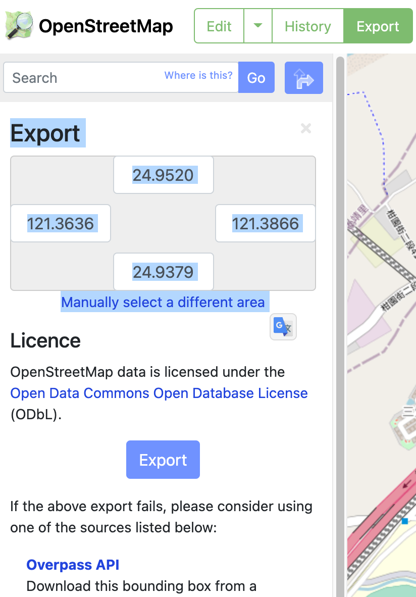
then:
mp$extract$osmBBox()
# then paste to get_stamenmap
6.4 Simple feature
install.packages("sf")Another type of geographic data structure.
a new class. Each value in a simple feature vector represents a form of geometry (called feature) and its geographic notation (i.e. latitude and longitude); and could carry its coordinate reference system.
Each value is a parsing result from
sf::st_xxxfunctions wherexxxcan bepoint(台北大學的一個地標,如YouBike站),multipoint(台北大學所有地標),linestring(台北大學的一條路徑),polygon(台北大學的一棟建築),multilinestring(台北大學的所有路徑),multipolygon(台北大學的所有建築), orgeometrycollection(整個台北大學)
6.4.1 Define simple features
A simple feature is composed of numeric vector, matrix, or list. No data frame is used.
geoValues <- list()
geoValues$simple_feature$point <-
  sf::st_point(
    c(24.9433123, 121.3699526)
  )
geoValues$simple_feature$multipoint <-
  sf::st_multipoint(
    rbind( # will form a matrix
      c(24.9443019, 121.3714944), # 1st point
      c(24.9440709, 121.3728518) # 2nd point
    )
  )
geoValues$simple_feature$linestring <-
  sf::st_linestring(
    rbind(
      c(24.9423755, 121.3679438), # 1st trace point
      c(24.9429941, 121.3679432), # 2nd trace point
      c(24.9432087, 121.3686713) # 3rd trace point
    )
  )
geoValues$simple_feature$polygon <-
  sf::st_polygon(
    list(
      # 1st closed trace
      rbind(
        c(24.9441895, 121.3695181),
        c(24.9442244, 121.3692544),
        c(24.9437158, 121.3694094),
        c(24.9438647, 121.3696271),
        c(24.9441895, 121.3695181) # close the polygon
      )
    )
  )
# polygon: a list consists of matrices.class(geoValues$simple_feature$point)
class(geoValues$simple_feature$linestring)
class(geoValues$simple_feature$polygon)
# all have sfg classSimple feature value can be graphed directly via geom_sf()
geoValues$simple_feature$polygon |> ggplot()+geom_sf()6.4.2 Form simple feature column
A collection column of multiple simple features.
sf::st_sfc(geoValues$simple_feature) -> geoValues$simple_feature_column

class(geoValues$simple_feature_column) # "sfc_GEOMETRY" "sfc"
# has class sfcgeoValues$simple_feature_column |>
ggplot()+geom_sf()6.4.3 Form simple feature data frame
- A simple feature data frame is basically a data frame with a column named geometry which is a list of each obervation’s simple feature value.
# initiate a data frame
df_sf <- data.frame(
  name=c("landmark 1", "must-see landmarks", "path 1", "building 1")
)

# add simple feature column
df_sf |> sf::st_set_geometry(geoValues$simple_feature_column) ->
  geoValues$simple_feature_df

class(df_sf) # only "data frame"
df_sf |>
  dplyr::mutate(
    geometry=geoValues$simple_feature_column
  ) -> df_sf2
class(df_sf2) # still a "data frame"
# Must go through sf::st_set_geometry to get sf class
class(geoValues$simple_feature_df) # "sf" "data.frame"

geoValues$simple_feature_df |> ggplot()+geom_sf()
6.5 Import Simple Feature Data
6.5.1 From SHP file
台灣的sf data太細,以平常輸出並不需要這麼細,可以進行簡化。使用:
sf_data |> mp$sf$simplify() -> sf_simplified_data6.5.2 From OSM
Define bounding box
Find feature key and value
Make open pass query to get sf data.
bbox = c(left = 121.0316, bottom = 24.7384, right = 122.1096, top = 25.3114) |>
  osmdata::opq() |>
  osmdata::add_osm_feature(key="admin_level", value="4") |>
osmdata::osmdata_sf() -> taipei_osm- If you have multiple features to request, chain
add_osm_features one after the other.
OR
bbox = c(left = 121.0316, bottom = 24.7384, right = 122.1096, top = 25.3114)
features = c("admin_level"="4")
mp$osm$request_data(
  bbox, features = features
) -> taipei_osm- features is a named character vector, with keys be element names and values be element values.
taipei_osm$osm_multipolygons |>
  dplyr::filter(name != "臺灣省") -> sf_northTaipei

sf_northTaipei |>
  ggplot()+geom_sf()

sf_northTaipei |>
  ggplot()+geom_sf(aes(fill=name))
6.5.3 sf overlay ggmap
Taipei MRT
bbox = c(left = 121.0316, bottom = 24.7384, right = 122.1096, top = 25.3114)
features = c("railway"= "subway")
mp$osm$request_data(
  bbox, features
) -> taipei_mrttaipei_mrt$osm_lines |>
ggplot()+geom_sf()# Error, since ggmap has some aes setting at the ggplot() stage which will be inherited by all the following geoms
taipei1()+
geom_sf(
data=taipei_mrt$osm_lines,
color="dodgerblue"
)taipei1()+
geom_sf(
data=taipei_mrt$osm_lines,
color="dodgerblue",
inherit.aes = FALSE
)sf overlay google map from ggmap might have problem. If it does, try the following tip:
6.5.4 data frame overlay ggmap
taipei_mrt$osm_lines |> sf::st_coordinates() -> coordinates
coordinates |> class()

taipei1() +
  geom_path(
    data=coordinates |> as.data.frame(),
    mapping=aes(
      x=X, y=Y, group=L1
    ),
    inherit.aes = FALSE
  )
6.6 Taiwan drug problem
sf_taiwan_simplified <- econDV2::sf_taiwan_simplified

sf_taiwan_simplified$台灣本島$縣市 |>
  ggplot()+geom_sf()
sf_taiwan_simplified$台灣本島$鄉鎮區 |>
  ggplot()+geom_sf()
Cast the geometry column to have uniform feature if your want to use plotly::ggplotly later:
# Originally polygons mixed with multipolygons
sf_taiwan_simplified$台灣本島$鄉鎮區 |> sf::st_geometry()

# re-cast to uniform multipolygon
sf_taiwan_simplified$台灣本島$鄉鎮區 |>
  sf::st_cast("MULTIPOLYGON") ->
  sf_taiwan_simplified$台灣本島$鄉鎮區
mp <- econDV2::Map()mp$sf$make_background_map底圖製作
6.6.1 縣市底圖
econDV2::Object(background)sf_taiwan_simplified$台灣本島$縣市 |>
mp$sf$make_background_map()
background$台灣本島$縣市 <- function(){
sf_taiwan_simplified$台灣本島$縣市 |>
mp$sf$make_background_map(
color="white",
size=0.14
)
}
background$台灣本島$縣市()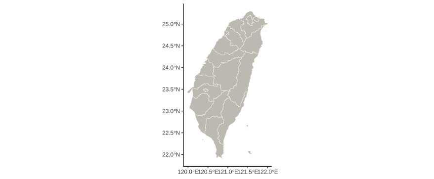
If you don’t know how much to crop and want to explore different possibilities, you can:
sf_taiwan_simplified$縣市 |>
  mp$sf$gg_crop()
6.6.2 各鄉/鎮/區底圖
background$台灣本島$鄉鎮區 <- function(){
  sf_taiwan_simplified$台灣本島$鄉鎮區 |>
    sf::st_cast("MULTIPOLYGON") |>
    mp$sf$make_background_map(
      color="white",
      size=0.14
    )
}

background$台灣本島$鄉鎮()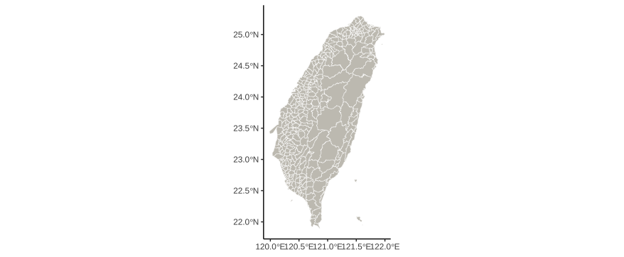
6.6.3 stamenmap底圖
bbox <- c(left=119.99690,
bottom=21.89988,
right=122.00000,
top=25.29999)econDV2::Object(taiwan_stamen)
# toner-lite
taiwan_stamen$tonerlite <-
ggmap::get_stamenmap(bbox, maptype="toner-lite", zoom=9)
background$台灣本島$tonerlite <-
function(){
ggmap::ggmap(taiwan_stamen$tonerlite)
}
background$`台灣本島`$tonerlite()
# terrain
taiwan_stamen$terrain <-
ggmap::get_stamenmap(bbox, maptype="terrain", zoom=9)
background$台灣本島$terrain <- function(){
ggmap::ggmap(taiwan_stamen$terrain,
darken=c("0.3", "white"))
}
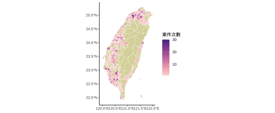
background$台灣本島$terrain()6.6.4 毒品破獲
創立帶有geometry column的sf毒品資料
繪製面量圖
econDV2::Object(drug)
drug$data <- jsonlite::fromJSON("https://www.dropbox.com/s/dry3nvahkmcmqoi/drug.json?dl=1")
drug$data <- drug$data |>
  dplyr::filter(發生西元年=="2018")
# 計算不同發生地點的案件破獲次數
library(dplyr)
drug$data |>
group_by(發生地點) |>
summarise(
案件次數=n(),
案件次數2=cut(案件次數, c(0, 10, 20, 30))
) -> drug$data_frequency6.6.4.2 overlay sf background
drug$map$choropleth0 <- function(){
  background$`台灣本島`$鄉鎮區() +
    geom_sf(
      data=drug$sf,
      mapping=aes(
        fill=案件次數
      ),
      color="white",
      size=0.15
    )
}

drug$map$choropleth0()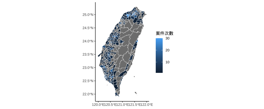
# mp$choose_palette()
drug$register_palette <- function(){
  colorspace::sequential_hcl(n = 3, h = c(-83, 20), c = c(65, NA, 18), l = c(32, 90), power = c(0.5, 1), rev = TRUE, register = "drug")
}

drug$register_palette()drug$map$choropleth0() +
colorspace::scale_fill_continuous_sequential(
palette="drug",
na.value="#dbd7a8"
)
drug$map$choropleth1 <- function(){
  background$`台灣本島`$鄉鎮區() +
    geom_sf(
      data=drug$sf,
      mapping=aes(
        fill=案件次數2,
        label=map_id
      ),
      color="white",
      size=0.15
    )
}drug$map$choropleth1() +
colorspace::scale_fill_discrete_sequential(
palette="drug",
na.value="#dbd7a8"
) +
theme_void() -> drug$map$choropleth_final
drug$map$choropleth_final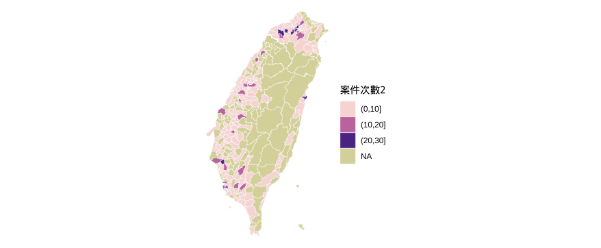
plotly::ggplotly(
  drug$map$choropleth_final
)
If you want to make the entire Taiwan island’s choropleth map down to “縣市” or “鄉鎮區,” you can also use:
econDV2::geom_sf_taiwanwhich only need social-econ data with map_id. It will create sf social-econ data in the background for you.econDV2::geom_sf_taiwandefault atcast2multipolygon=Tto ensureplotly::ggplotlywork.
ggplot()+
  econDV2::geom_sf_taiwan(
    data=drug$data_frequency,
    mapping=aes(
      fill=案件次數
    ),
    map_id = "發生地點",
    type="鄉鎮區"
  )

last_plot() +
  colorspace::scale_fill_continuous_sequential(
    palette="drug",
    na.value="#dbd7a8"
  )

plotly::ggplotly(last_plot())- background map design change is also possible.
ggplot()+
  econDV2::geom_sf_taiwan(
    data=drug$data_frequency,
    mapping=aes(
      fill=案件次數2
    ),
    color="white",
    size=0.15,
    map_id = "發生地點",
    type="鄉鎮區",
    background.fill = "#ebffd9",
    background.color = "#d9d9d9",
    background.size = 0.1
  )

last_plot() +
  colorspace::scale_fill_discrete_sequential(
    palette="drug",
    na.value="#dbd7a8"
  ) +
  theme_void()

plotly::ggplotly(last_plot())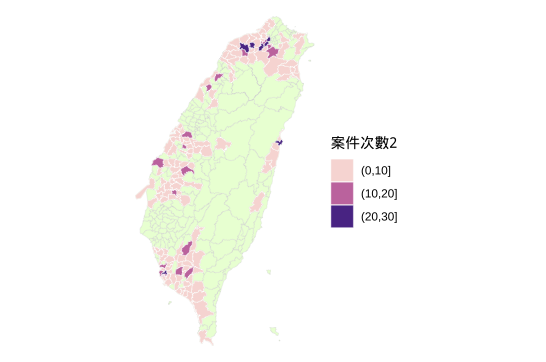
6.6.4.3 overlay stamenmap background
drug$map$overstamen_tonerlite <-
  background$`台灣本島`$tonerlite() +
    geom_sf(
      data=drug$sf,
      mapping=aes(
        fill=案件次數2,
        label=map_id
      ),
      color="white",
      size=0.15,
      alpha=0.3,
      inherit.aes = F
    ) +
  colorspace::scale_fill_discrete_sequential(
    palette="drug",
    na.value=ggplot2::alpha("#dbd7a8", 0.1)
  )

drug$map$overstamen_tonerliteplotly::ggplotly(drug$map$overstamen_tonerlite)- The overlay is slightly off due to some bug in ggmap. To fix it, you can use
econDV2::ggmap2() + econDV2::geom_sf_overggmap()
drug$map$overstamen_tonerlite_fixed <-
  econDV2::ggmap2(taiwan_stamen$tonerlite)+
    econDV2::geom_sf_overggmap(
        data=drug$sf,
        mapping=aes(
          fill=案件次數2,
          label=map_id
        ),
        color="white",
        size=0.15,
        alpha=0.7,
        inherit.aes = F
      ) +
    colorspace::scale_fill_discrete_sequential(
      palette="drug",
      na.value=ggplot2::alpha("#dbd7a8", 0.1)
    )+theme_void()

drug$map$overstamen_tonerlite_fixed

plotly::ggplotly(drug$map$overstamen_tonerlite_fixed)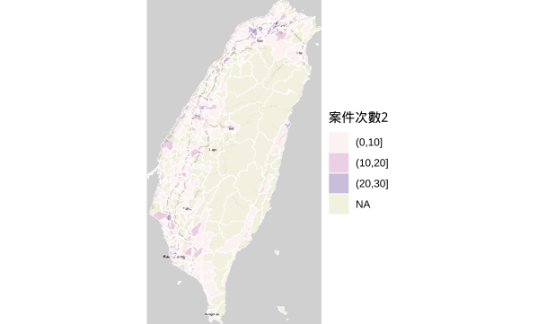
- There is still some unfit due to the fact that sf geometry is simplified.
Terrain
drug$map$overstamen_terrain <-
  background$`台灣本島`$terrain() +
    geom_sf(
      data=drug$sf,
      mapping=aes(
        fill=案件次數2,
        label=map_id
      ),
      color="white",
      size=0.15,
      alpha=0.7,
      inherit.aes = F
    ) +
  colorspace::scale_fill_discrete_sequential(
    palette="drug",
    na.value=ggplot2::alpha("#dbd7a8", 0.1)
  )

drug$map$overstamen_terraindrug$map$overstamen_terrain_fixed <-
econDV2::ggmap2(taiwan_stamen$terrain) +
econDV2::geom_sf_overggmap(
data=drug$sf,
mapping=aes(
fill=案件次數2,
label=map_id
),
color="white",
size=0.15,
alpha=0.5,
inherit.aes = F
) +
colorspace::scale_fill_discrete_sequential(
palette="drug",
na.value=ggplot2::alpha("#dbd7a8", 0.1)
)+theme_void()
drug$map$overstamen_terrain_fixed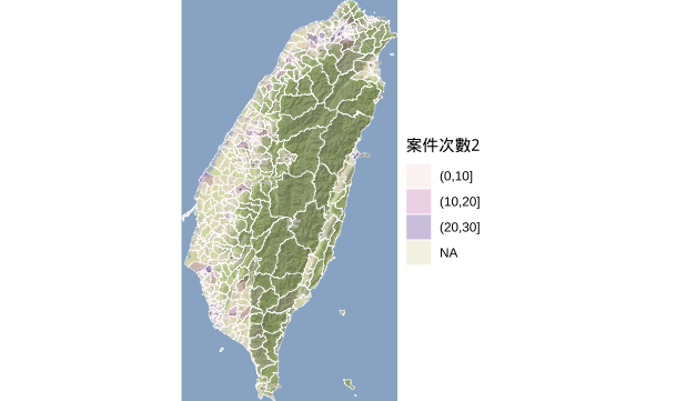
plotly::ggplotly(drug$map$overstamen_terrain_fixed)