第 4 章 Categorical data

4.1 Aesthetics: group

ggplot() +
  geom_line(
    mapping=aes(
      x=c(1, 2, 3),
      y=c(2, 3, 2),
    )
  ) +
  geom_line(
    mapping=aes(
      x=c(1, 2, 3),
      y=c(5, 2, 6)
    )
  )

Use group aesthetic to combine

multiple same geom layers

into one.

ggplot() +
  geom_line(
    mapping=aes(
      x=c(1, 2, 3, 1, 2, 3),
      y=c(2, 3, 2, 5, 2, 6),
      group=c("m", "m", "m", "f", "f", "f"), 
    )
  )

ggplot() +
  geom_line(
    mapping=aes(
      x=c(1, 2, 3, 1, 2, 3),
      y=c(2, 3, 2, 5, 2, 6),
      group=c("m", "m", "m", "f", "f", "f"),
      color=c("m", "m", "m", "f", "f", "f")
    )
  )

Any aesthetic differentiates group can replace group.

ggplot() +
  geom_line(
    mapping=aes(
      x=c(1, 2, 3, 1, 2, 3),
      y=c(2, 3, 2, 5, 2, 6),
      # group=c("m", "m", "m", "f", "f", "f"),
      color=c("m", "m", "m", "f", "f", "f")
    )
  )

When there is no aesthetic mapping to differentiate groups, use group aesthetic mapping.

4.2 Geom overlapping

When geom layers overlap, we can use

alpha aesthetic.

If multiple geometries are created within the one geom_ call (using grouping aesthetics), we can also set

position: “stack,” “dodge” or “jitter” (some of them might not apply to certain geom_)

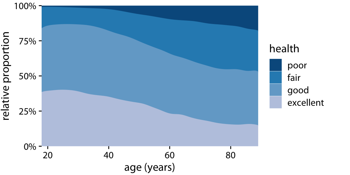
https://clauswilke.com/dataviz/visualizing-proportions.html#fig:health-vs-age
x is continuous, or discrete with many types
y the cumulative proportion

ggplot() +
  geom_area(
    mapping=aes(
      x=c(1, 2, 3),
      y=c(0.2, 0.3, 0.2),
    )
  ) +
  geom_area(
    mapping=aes(
      x=c(1, 2, 3),
      y=c(0.4, 0.3, 0.52) + c(0.2, 0.3, 0.2) # the additive is for accumulative purpose
    ), 
    alpha=0.5
  )

4.3 Position: stack

put y on top of the overlapping geom’s y
create accumulative result.

ggplot() +
  geom_area(
    mapping=aes(
      x=c(1, 2, 3, 
        1, 2, 3),
      y=c(0.2, 0.3, 0.2, 
        0.4, 0.3, 0.52),
      fill=c("m", "m", "m", 
        "f", "f", "f")
    ),
    position="stack" #input$position
  )

stack position is accumulative; no need to compute the accumulative value yourself.
the default position in geom_area is “stack.” Therefore, you can omit position argument.

data_cat1 <- data.frame(
      x=c(1, 2, 3, 1, 2, 3),
      y=c(0.2, 0.3, 0.2, 0.4, 0.4, 0.52),
      fill=c("m", "m", "m", "f", "f", "f")
)

ggplot(
  data=data_cat1
) + 
  geom_area(
    mapping=aes(
      x=x,
      y=y,
      fill=fill
    )
  )

When aesthetic mapping involves with unordered data, it will

convert the data series into factor (unless the series is already a factor);
conduct the mapping according to the level sequence of the converted factor.

data_cat1$fill |>
  factor() |>
  levels()

4.4 Factor

When grouping aesthetics vary the look of geometries across different groups of data, it is crucial that users declare the mapped series with proper class.

factor(data_series, levels) parses data_series into a categorical data with expressing sequence defined by levels.
If omit levels the level sequence will be determined by the collateral sequence defined by your operating system.

ggplot(
  data=data_cat1
) + 
  geom_area(
    mapping=aes(
      x=x,
      y=y,
      fill=factor(fill, levels=c("m", "f"))
    )
  )

Here we declare factor on-the-go.

We can also declare factor in the data frame first:

data_cat1_copy <- data_cat1
data_cat1_copy$fill |>
  factor(levels=c("m", "f")) -> 
  data_cat1_copy$fill

|> is a R 4.0+ equipped operator, which makes:

f(x, ....) # equivalent to
x |> f(...)

ggplot(
  data=data_cat1_copy
) + 
  geom_area(
    mapping=aes(
      x=x,
      y=y,
      fill=fill
    )
  )

4.5 Proportional data

data_cat2_wide <- data.frame(
      x=c(1, 2, 3),
      y_a=c(0.2, 0.3, 0.2),
      y_b=c(0.4, 0.4, 0.52),
      y_c=c(0.4, 0.3, 0.28)
)

data_cat2_wide |> 
  tidyr::pivot_longer(
    cols=y_a:y_c,
    names_to = "fill",
    values_to= "y"
  ) ->
  data_cat2

View(data_cat2)

ggplot(
  data=data_cat2
) + 
  geom_area(
    mapping=aes(
      x=x,
      y=y,
      fill=fill
    ),
    color="white"
  )

When x mapping series has limited cases and is discrete, a bar chart with position dodge is better.

ggplot(
  data=data_cat2
) + 
  geom_col(
    mapping=aes(
      x=x,
      y=y,
      fill=fill
    ),
    color="white",
    width=0.8, #input$width
    size=0, #input$size
    position = "dodge" #input$position
  )

width: the width of the bar
size: the size of the stroke

Pie chart:

not good for comparing proportion across more than one dimension

library(dplyr)
data_cat2 %>%
  filter(
    x==1
  ) -> 
  data_cat2_x1only

ggplot(
  data=data_cat2_x1only
) + 
  geom_col(
    aes(
      x=x,
      y=y,
      fill=fill
    )
  )

ggplot(
  data=data_cat2_x1only
) + 
  geom_col(
    aes(
      x=x,
      y=y,
      fill=fill
    )
  ) +
  coord_polar(
    theta = "y"
  )

4.6 Adding text

adding text

ggplot(
  data=data_cat2_x1only
) + 
  geom_col(
    aes(
      x=x,
      y=y,
      fill=fill
    )
  ) +
  geom_text(
    aes(
      x=x,
      y=y,
      label=fill
    ),
    position = "stack"
  )

geom_col stack sequence is based on fill level sequence.
geom_text stack sequence is based on observation sequence.

Grouping aesthetics determine the sequence of stacking. In geom_col, fill is the grouping aesthetic. To make geom_text stack labels in sequence as fill in geom_col, we can put group=fill in geom_text to create such a sequence.

ggplot(
  data=data_cat2_x1only
) + 
  geom_col(
    aes(
      x=x,
      y=y,
      fill=fill
    )
  ) +
  geom_text(
    aes(
      x=x,
      y=y,
      label=fill,
      group=fill
    ),
    position = "stack"
  )

Change labels to represent the proportion values of y

ggplot(
  data=data_cat2_x1only
) + 
  geom_col(
    aes(
      x=x,
      y=y,
      fill=fill
    )
  ) +
  geom_text(
    aes(
      x=x,
      y=y,
      label=y, # use y to label now
      group=fill
    ),
    position = "stack"
  )

position argument also takes position functions.
When you know what type of position you want, you can use corresponding position function to fine tune the position.

ggplot(
  data=data_cat2_x1only
) + 
  geom_col(
    aes(
      x=x,
      y=y,
      fill=fill
    )
  ) +
  geom_text(
    aes(
      x=x,
      y=y,
      label=y,
      group=fill
    ),
    position = position_stack(vjust=0.5)
  )

ggplot(
  data=data_cat2_x1only
) + 
  geom_col(
    aes(
      x=x,
      y=y,
      fill=fill
    )
  ) +
  geom_text(
    aes(
      x=x,
      y=y,
      label=y,
      group=fill
    ),
    position = position_stack(vjust=0.5)
  ) +
  coord_polar(
    theta = "y"
  ) +
  theme_void()

When x-axis is also representing a categorical data:

dy=0.03 # input$dy
ggplot(
  data=data_cat2
) + 
  geom_col(
    mapping=aes(
      x=x,
      y=y,
      fill=fill
    ),
    color="white",
    width=0.8, #input$width
    position = "dodge" #input$position
  )+
  geom_text(
    mapping=aes(
      x=x,
      y=y-dy,
      group=fill,
      label=y
    ),
    size=8, #input$size
    position=position_dodge(width=
        0.8 #input$dodge
        )
  )

text position_dodge has the same width as geom_col to ensure the same dodging distance.

4.7 More on position

https://ggplot2.tidyverse.org/reference/index.html#section-position-adjustment

4.8 Coordination flip

ggplot()+
  geom_col(
    mapping=
      aes(
        x=c("A", "B", "C"),
        y=c(56, 77, 92)
      )
  )+
  coord_flip()

Another common application of coord_flip is:

dx=4 #input$dx
h=0.5 #input$h
dt=0 #input$dt
ggplot()+
  geom_col(
    mapping=aes(
      x=c(1, 1),
      y=c(306, 232),
      fill=c("biden","trump")
    ),
    width=1
  )+
  geom_segment(
    mapping=aes(
      x=1-h,
      y=270,
      xend=1+h,
      yend=270
    )
  )+
  geom_text(
    mapping=aes(
      x=1+dt,
      y=270,
      label="270"
    ),
    size=8 #input$text
  )+
  xlim(1-dx, 1+dx)+ # make sure cover 0.5-1.5 so the bar width can be accomodate
  coord_flip()+
  theme_void()+
  theme(legend.position = "none")

4.9 Summary

Grouping aesthetic separate a data frame into various subsample data frame and apply the geom_ function to each one of them in the sequence determined by the mapping factor’s levels sequence.
When group aesthetic and other aesthetic share the same mapping variable, group aesthetic can be ignored.
When deal with grouping variable, values of y from different groups at the same x can have position choice:
- “identity”: respect ys as it is.
- “stack”: stack ys according to grouping level sequence.
- “dodge”: respect ys as it is but move their x values left and right according to grouping level sequence.

Economic Data Visualization