Chapter 6 Optimization
6.1 Module
- A module is a file containing code, or called source code.
# R
xfun::download_file("https://www.dropbox.com/s/49y23ib21ncylyh/consumer.R?dl=1")
# Py
xfun::download_file("https://www.dropbox.com/s/u05jezbxt99z8ho/consumer.py?dl=1")
6.1.1 Where to put
- If the module is only for the current project:
Place all the modules used by a Python program in the same directory as the program – if called from Rmd, it means the directory of the Rmd file. Inside your Rmd, run the following to get this path:
getwd() # if you run xfun::download_file within Rmd, your module/source file should be at thie directory already.- If the module is for general purpose and to be used in several projects:
Create a directory (or directories) to hold your modules, and for Python modify the sys.path variable so that it includes this new directory (or directories), and for R you don’t have to setup anything.
sys.path.extend(['/Users/martinl/Dropbox/github-data/109-2-P4Economic_Model'])6.1.2 Import your module
Source your source script:
source("/Users/martinl/Dropbox/github-data/109-2-P4Economic_Model/consumer.R")consumer11 <- Consumer(c(1,1)) # preference: x*y
consumer35 <- Consumer(c(3,5)) # preference: x**3 * y**5Import your module script:
import consumer
import consumer as cs # create an acronym for easy module access

consumer0 = cs.Consumer((3,7))
consumer1 = consumer.Consumer((5,5))
python: importlook for the module file named consumer.py first at the project directory, thensys.path.
If you change your module on disk, retyping the import command won’t cause it to load again. You need to use the reload function from the imp module for this. The imp module provides an interface to the mechanisms behind importing modules:
import consumer

# If you update your module and want to reload:
import importlib as lib
lib.reload(consumer)
6.2 Optimization tools
6.2.1 R:optim
?optimoptim(par, fn, ...)Arguments
- par: Initial values for the parameters to be optimized over.
- fn: A function to be minimized (or maximized), with first argument the vector of parameters over which minimization is to take place. It should return a scalar result.
fr <- function(x) {   ## Rosenbrock Banana function
    x1 <- x[1]
    x2 <- x[2]
    100 * (x2 - x1 * x1)^2 + (1 - x1)^2
}
optim(c(-1.2, 1), fr)
6.2.2 Python:scipy.optimize
from scipy import optimize
import numpy as np

help(optimize.minimize)
minimize(fun, x0, args=(), method=None, jac=None, hess=None, hessp=None, bounds=None, constraints=(), tol=None, callback=None, options=None)
Minimization of scalar function of one or more variables.
Parameters
----------
fun : callable
The objective function to be minimized.
``fun(x, *args) -> float``
where ``x`` is an 1-D array with shape (n,) and ``args``
is a tuple of the fixed parameters needed to completely
specify the function.
x0 : ndarray, shape (n,)
Initial guess. Array of real elements of size (n,),
where 'n' is the number of independent variables.
args : tuple, optional
Extra arguments passed to the objective function and its
derivatives (`fun`, `jac` and `hess` functions).6.3 Array
dimension
data type
6.3.1 Dimension
1-D: \[\left[\begin{array}{cc} 1.1 & 1.2 \end{array}\right]\]
mat_1d = c(1.1, 1.2)mat_1d = np.array([1.1, 1.2])
print(mat_1d)2-D: \[\left[\begin{array}{cc} 1.1 & 1.2\\ 2.1 & 2.2\\ 3.1 & 3.2\\ 4.1 & 4.2 \end{array}\right]\]
mat_2d = rbind(
  c(1.1, 1.2),
  c(2.1, 2.2),
  c(3.1, 3.2)
)

print(mat_2d)
mat_2d = np.array(
[
[1.1, 1.2],
[2.1, 2.2],
[3.1, 3.2]
]
)
print(mat_2d)mat_1d
mat_1d.ndim # 1 維- Notice 1-D array must have shape
(D,). If put it(D,1), it will turn into a 2 dimensional array where 2 comes from the length of(D,1)tuple.
.shape attribute when changed will change the way the array print on the screen.
mat_2d
mat_2d.ndim  # 2 維
mat_2d.shape # 3 x 2
array([[1.1, 1.2],
[2.1, 2.2],
[3.1, 3.2]])Now:
mat_2d.shape = (2,3) # OR
mat_2d.reshape(2,3)
mat_2d
array([[1.1, 1.2, 2.1],
[2.2, 3.1, 3.2]])Another common shape changer is transpose of a matrix:
mat_2d.transpose()array([[1.1, 2.1, 3.1],
[1.2, 2.2, 3.2]])mat_1d1 = np.array([2])
mat_1d2 = np.array([3,5])
mat_1d_stack = np.hstack(
(mat_1d1, mat_1d2) # arrays to be stacked should be placed inside a tuple
)6.3.2 Data type
R matrix consists of atomic vectors. All elements have the same data type. Python does not have atomic vectors; all vectors can have elements of heterogeneous data types. numpy ensures that all arrays have homogeneous elements as R.
mat_1d.dtype
mat_2d.dtype
Proper dtype to make program more efficient.
mat_1d_dtype1 = np.array([2, 3]) # int default int64
mat_1d_dtype1.dtype

mat_1d_dtype2 = np.array([2, 3], dtype='int32')
mat_1d_dtype2.dtype

mat_1d_dtype3 = np.array([2, 3], dtype='float32')
mat_1d_dtype3.dtype

mat_1d_dtype4 = np.array([2, 3], dtype='float64') # float default
mat_1d_dtype4.dtype
6.3.3 Refitting preference function
old preference:
def preference(x, params):
    assert type(x) is tuple, "x should be a tuple"
    assert type(params) is tuple, "params should be a tuple"
    x1, x2 = x
    alpha, beta = params
    u = x1**alpha * x2**beta
    return u

# EOFpreference((3,5), (0.2, 0.8))def preference_refit(x, params):
assert type(x) is np.ndarray, "x should be an 1-d ndarry"
assert type(params) is tuple, "params should be a tuple"
alpha, beta = params
x1, x2 = x
u = x1**alpha * x2**beta
return u
# EOFpreference_refit(
mat_1d, (0.2, 0.8)
)- Has to redesign preference each time.
6.4 Function generator
f_gen <- function(fn, ...){

  new_function <- function(...){
    fn # outside input can be used here
  }

  return(new_function)
}
def f_gen(fn, ...):
def new_function(...):
fn # outside-input can be used here
return something
return new_functionHousehold utilities:
\[U_h(x, \alpha_h)=x_1^{\alpha_h}*x_2^{1-\alpha_h},\] \[U_w(x, \alpha_w)=x_1^{\alpha_w}*x_2^{1-\alpha_w},\] Household aggregate utility: \[U(x, \gamma)=U_h(x)^{\gamma}*U_w(x)^{1-\gamma}\]
U_household <- function(Uh, Uw){
  householdU <- function(x, gamma){ # the returned function input reflects the household utility inputs
    Uh(x)**gamma * Uw(x)**gamma # any objects you need to completes the returned value should be the inputs from the outside-function inputs
  }
  return(householdU)
}
U_h <- function(x, alpha=0.2) x[[1]]**alpha * x[[2]]**(1-alpha)
U_w <- function(x, alpha=0.7) x[[1]]**alpha * x[[2]]**(1-alpha)
U_h(c(2, 3))
U_w(c(2, 3))
U_whenMarried <- U_household(Uh=U_h, Uw=U_w)
U_whenMarried(c(2, 3), gamma=0.3)def U_household(Uh, Uw):
def householdU(x, gamma): # the returned function input reflects the household utility inputs
uh = Uh(x)**gamma * Uw(x)**gamma # any objects you need to completes the returned value should be the inputs from the outside-function inputs
return uh
return householdU
# EOFdef U_h(x, alpha=0.2): return x[0]**alpha * x[1]**(1-alpha)
def U_w(x, alpha=0.7): return x[0]**alpha * x[1]**(1-alpha)
U_h((2, 3))
U_w((2, 3))
U_whenMarried = U_household(Uh=U_h, Uw=U_w)
U_whenMarried((2, 3), gamma=0.3)In the example above, U_h and U_w have the same type of function; they only differ at alpha. Write a U_genByAlpha function such that:
U_h = U_genByAlpha(alpha=0.2)
U_w = U_genByAlpha(alpha=0.7)

U_h((2, 3))
U_w((2, 3))
The output is a function that takes only x value and no default of alpha (it is already set when generated by U_genByAlpha)
Our goal:
- design
convert2objectivefunction such that whenpreferencefunction is input, the returned is a new preference function that can take 1-D array as its first input:
preference_refit2 = convert2objective(preference)

mat_1d = np.array([1.1, 1.2])
preference_refit2(mat_1d, (0.2, 0.8))
def convert2objective(preference):
# image a new function that takes in x and params as the type you want. But you can only use function preference() to generate utility:
def obj(x, params):
x = tuple(x)
return preference(x, params)
# return function as an output
return obj
# EOF6.4.1 Let’s optimize
def f(x):
    return 2*(x-3)**2

# EOF
x0 = np.array([5])
f(x0) # check if f works on np.ndarrayf_optimized = optimize.minimize(f, x0)
print(f_optimized)
f_optimized.x # solutionYou might notice that the optimal solution is 2.9999x instead of true minimum, 3. This is what differentiates “numerical solution(數值求解)” (2.9999x) from “analytical solution(分析求解)” (3). Numerical solutions often rely on numerically differentiating a function as the exercise I gave in R introduction course. Error is introduced already in that stage. Therefore, even we know interior solution must have its first derivative equal to zero. In numerical practice, numerical differentiation may never yield that outcome.
Other than that, numerical solution recursively lands on a “decent” solution based on some converging criterion, which is often expressed as “if the numerical first differential is smaller than some small number, then computer can stop.” This “some small number” is one parameter that governs the degree of accuracy. Completely equal to zero is not practical for numerical purpose, which will drag your solution search, and trap computer in some impractically long runtime.
However, when accuracy requirement is important for you, you could possibly reach extreme accuracy via:
supplying function’s first derivative function manually. Feed in analytically accurate derivative function can heavily increase accuracy. However, for general purpose, hand compute analytical first derivative might be impossible.
using a better hardware.
You might ask what about the second order derivative. Yes, supply it analytically helps too. Researchers call this type of solution improvement second degree improvements–in contrast to the first degree improvement from explicitly supplying first derivative function.
6.5 Minimization with constraint
Express all inequality constraint into non-negative constraint:
\[2*x+3*y \leq 500\] In non-negative expression: \[500-2*x-3*y \geq 0\]
def const_nonNeg(x,y):
    return 500-2*x-3*y
\[ \begin{align*} \max_{\{x,y\}}U(x,y) & \equiv x^{0.2}y^{0.8}\\ s.t.\ & 2x+3y\leq500 \end{align*} \]
def U(x,y):
  return -(x**0.2 * y**0.8) # take negative for minimization purpose
For scipy::minimize, all function input must be a (n,) array, including U and const_nonNeg.
def convert2arrayInputFunction(f0):
   def newFun(x_array):
       return f0(*x_array)
return newFun*tupleor*listwill unpack tuple or list into inputs likeinput1, input2, input3for feeding into a function call for these unpacked inputs, likef(input1, input2, input3)
newU = convert2arrayInputFunction(U)
newConst_nonNeg = convert2arrayInputFunction(const_nonNeg)

x = np.array([2,3])
newU(x)
newConst_nonNeg(x)
const_dict = ({ "type": "ineq", # change to "eq" for equality constraint
"fun": newConst_nonNeg
})- If multiple constraints, use
( {constraint1}, {constraint2}, ...., {contraintN})
x0 = np.array([1,1])

optimize.minimize(
  fun = newU, x0=x0,
  constraints= const_dict
)
Define a Consumer class that has:
Utility function like \(U(x,y)=x^{\alpha}*y^{1-\alpha}\).
Facing a budget constraint \(P_x*x+P_y*y\leq I\).
params_A = (0.2, 500) # (alpha, I)
consumer_A = Consumer(params)

params_B = (0.8, 200)
consumer_B = Consumer(params)

consumer_A.prices # (2, 3)
consumer_B.prices # both show market prices

c0 = (2,3)
consumer_A.U(c0)
consumer_B.U(c0) # show utilities of c0 for both consuemrs

consumer_A.optimise()
consumer_B.optimise() # show the optimisation result, and afterward

consumer_A.c_optim
consumer_B.c_optim # show the optimised c bundle

Consumer.prices = (5, 8)
consumer_A.optimise()
consumer_B.optimise() # show the optimisation result, and afterward

consumer_A.c_optim
consumer_B.c_optim # show the optimised c bundle

consumer_A.I = 300
consumer_A.optimise()
consumer_A.c_optim
6.6 Class method

Once upon a time, there were 500 consumers. Each had a linear individual demand \(qd(p)\) like:
\[qd(p)=\alpha-\beta*p,\] where \(\alpha, \beta > 0\) and \(qd(p)=0\) if \(\alpha-\beta*p<0\). These 500 consumers were created by god Zeus who randomly drew 500 pairs of \((\alpha, \beta)\) with \(\alpha\sim uniform(300, 500)\) and \(\beta \sim uniform(20, 100)\).
Historian discovered the following codes which were believed to be what Zeus used to create these 500 consumers:
from numpy.random import default_rng
rng_alpha = default_rng(2020)
rng_beta = default_rng(2022)

consumers500 = [ Consumer(alpha, beta) for alpha, beta in zip(rng_alpha.uniform(300,500, size=500), rng_beta.uniform(20, 100, size=500))]
It is believed that Zeus used the magic wand Consumder (a class generator) to create these 500 people.
def qd_generator(alpha, beta):
    def qd(p):
        return max(0, alpha-beta*p)
    return qd

class Consumer:
    def __init__(self, alpha, beta):
        self.alpha=alpha
        self.beta=beta
        self.qd = qd_generator(alpha, beta)
consumer300_20 = Consumer(300,20)
consumer450_40 = Consumer(450,40)
consumer300_20.qd(5)
consumer450_40.qd(5)Later historians discovered the following scripts:
Consumer.Qd(5) # this shows the total quantity demanded from numpy.random import default_rng
def qd_generator(alpha, beta):
def qd(p):
return max(0, alpha-beta*p)
return qd
class Consumer:
def __init__(self, alpha, beta):
self.alpha=alpha
self.beta=beta
self.qd = qd_generator(alpha, beta)
rng_alpha = default_rng(2020)
rng_beta = default_rng(2022)
consumers500 = [ Consumer(alpha, beta) for alpha, beta in zip(rng_alpha.uniform(300,500, size=500), rng_beta.uniform(20, 100, size=500))]The first guess is:
def Qd(p):
    total_q = sum([consumers500[i].qd(p) for i in range(len(consumers500))])
return total_qQd(5)However, Consumer.Qd(5) implies that Qd is a method defined inside Consumer:
class Consumer:
    def __init__(self, alpha, beta):
        self.alpha=alpha
        self.beta=beta
        self.qd = qd_generator(alpha, beta)

    def Qd(p):
        total_q = sum([consumers500[i].qd(p) for i in range(len(consumers500))])
        return total_q
There are two things need to take care:
Qd(p)does not depend onself. It should be a static method.Secondly,
consumers500is not defined when no consumer was created (though Zeus almighty might already knows). It should be a class variable.
class Consumer:

    consumers500 = []

    def __init__(self, alpha, beta):
        self.alpha=alpha
        self.beta=beta
        self.qd = qd_generator(alpha, beta)

    @staticmethod

    def Qd(p):
        total_q = sum([Consumer.consumers500[i].qd(p) for i in range(len(consumers500))])
        return total_q
The problem is the
Consumer.consumers500will always be empty.We need that: whenever a consumer instance is initiated, this consumer is added to
Consumer.consumers500.
Class variable that needs to be changed when an instance is initiated and be built into the __init__ method:
class Consumer:

    consumers500 = []

    def __init__(self, alpha, beta):
        self.alpha=alpha
        self.beta=beta
        self.qd = qd_generator(alpha, beta)
        Consumer.consumers500.append(self)
        # some prefer self.__class__.consumers500.append(self)

    @staticmethod

    def Qd(p):
        total_q = sum([Consumer.consumers500[i].qd(p) for i in range(len(Consumer.consumers500))])
        return total_q
consumer1 = Consumer(300, 10)
# Check the 1st consumer in consumer500 is really consumer1
Consumer.consumers500[0].alpha
Consumer.consumers500[0].beta
Consumer.consumers500[0].qd(2) # individual demand
# Aggregate demand
Consumer.Qd(2)
consumer2 = Consumer(500, 30)
# Check the 2nd consumer in consumer500 is really consumer2
Consumer.consumers500[1].alpha
Consumer.consumers500[1].beta
Consumer.consumers500[1].qd(2) # individual demand
# Aggregate demand
Consumer.Qd(2)Static method often involves with class variable, which needs to be writtend as {classname}.{classvariable}. Another approach is to use class method which like __init__ method for an instance that passes self as its first input; class method passes cls as its first input and access to a class variable can be doen via cls.{classvariable}:
def qd_generator(alpha, beta):
    def qd(p):
        return max(0, alpha-beta*p)
    return qd

class Consumer:

    consumers500 = []

    def __init__(self, alpha, beta):
        self.alpha=alpha
        self.beta=beta
        self.qd = qd_generator(alpha, beta)
        Consumer.consumers500.append(self)
        # some prefer self.__class__.consumers500.append(self)

    @classmethod # notice the declaration of classmethod

    def Qd(cls, p): # add cls to its first input
        total_q = sum([cls.consumers500[i].qd(p) for i in range(len(cls.consumers500))])
return total_q- Using class method is better than static method in the sense that if you decide to change your class name from Consumer to Household, you don’t have to change any Consumer object inside the class definition.
6.7 Into R realm
Goal: prepare a sequence of \((p, q)\) and \((p, Q)\) data for us to draw individual demands and aggregate demand in R.
p = 1
qds_at_p = [[i, p, consumer_i.qd(p)] for i, consumer_i in enumerate(consumers500)]
print(qds_at_p[0:5])
enumerate() turns an iterable object to an iterable that can emit each iterate’s index count.
- Here this index can serve as an id for panel data.
6.7.1 Pandas
import pandas as pd

pd_qds = pd.DataFrame(qds_at_p)
print(pd_qds)
import pandas as pd
def pd_qdsGenerator(p):
qds_at_p = [[i, p, consumer_i.qd(p)] for i, consumer_i in enumerate(consumers500)]
pd_qds = pd.DataFrame(qds_at_p, columns = ["ID","price","quantity"])
return pd_qdspd_qds_1 = pd_qdsGenerator(1)
pd_qds_2 = pd_qdsGenerator(2)
pd_qds_allP = pd.concat([pd_qds_1, pd_qds_2])
print(pd_qds_1)
print(pd_qds_2)
print(pd_qds_allP)6.7.2 Visualization
library(ggplot2)
library(dplyr)py$pd_qds_allP %>%
group_by(price) %>%
summarise(
quantity = mean(quantity)
) -> pd_Qds_meanPython codes executed under R with the help of reticulate package will create a py object in R realm that binds all Python results for R to access.
ggplot(data = py$pd_qds_allP) +
geom_line(
aes(
group=ID, x=quantity, y=price
), alpha=0.1
)+
geom_line(
data=pd_Qds_mean,
aes(x=quantity, y=price), color="dodgerblue3",
size=2
)+
theme_classic() -> gg_demands
gg_demands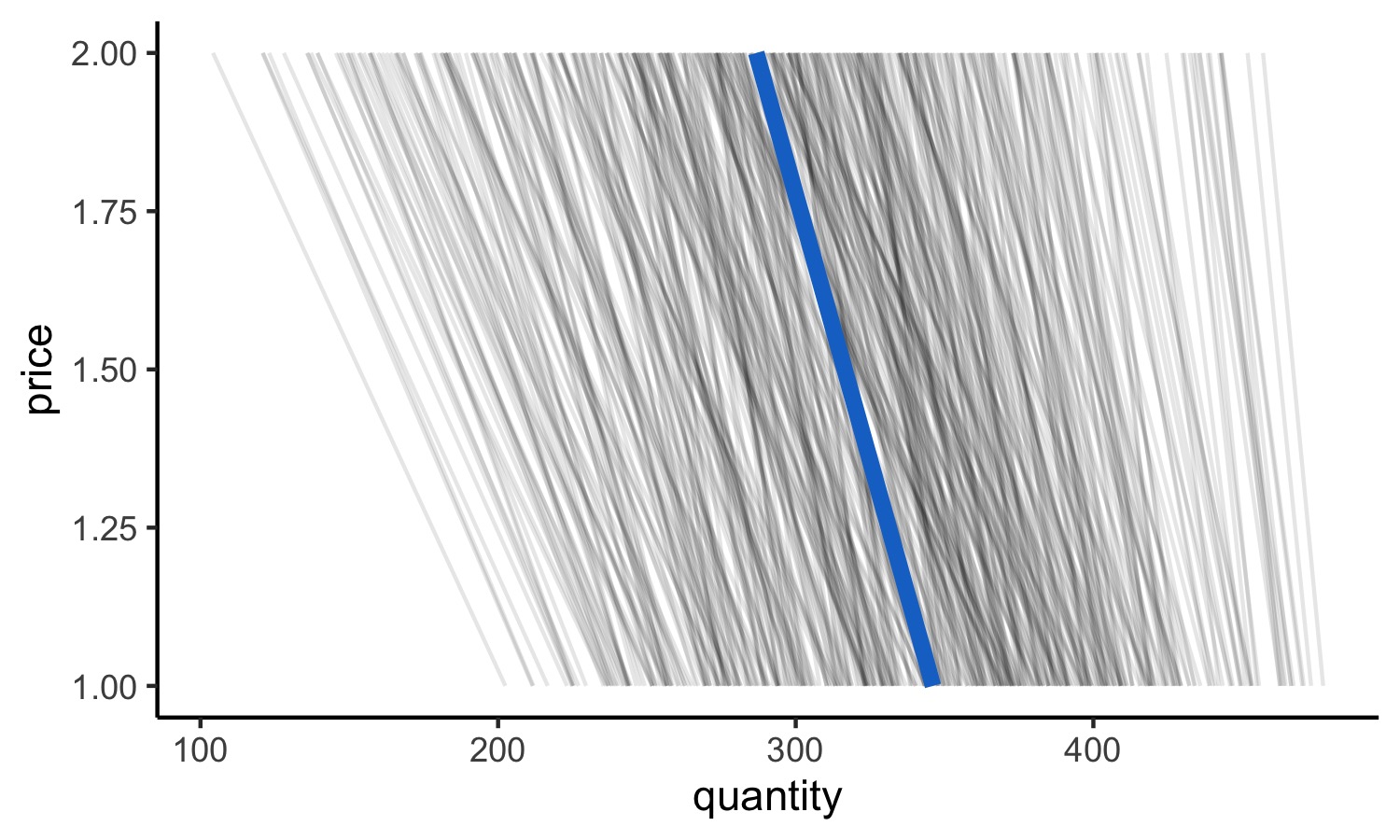
6.7.3 Integration
xfun::download_file("https://www.dropbox.com/s/cyp43ve6wyqnof1/consumers.py?dl=1", mode="wb")reticulate::source_python can source .py script as base::source can source .R script:
library(reticulate)
library(dplyr)
library(ggplot2)
reticulate::source_python(
"consumers.py"
)
py$pd_qds_allP %>%
  group_by(price) %>%
  summarise(
    quantity = mean(quantity)
  ) -> pd_Qds_mean
ggplot(data = py$pd_qds_allP) +
  geom_line(
    aes(
      group=ID, x=quantity, y=price
    ), alpha=0.1
  )+
  geom_line(
    data=pd_Qds_mean,
    aes(x=quantity, y=price), color="dodgerblue3",
    size=2
  )+
  theme_classic() -> gg_demands
gg_demands