第 2 章 Geometries and Aesthetics
Two steps:
Step 1: What geometries do you see?
Step 2: With a given geometry, what aesthetics do you observe?

Geometries?
Aesthetics?
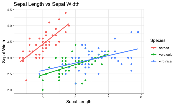

2.1 An Example

Geom:
geom_point:x, y:varies with observations
color (線框顏色): constant
stroke (線框粗細): constant
fill (內部塗色): constant
size (點的大小): constant
x, y: varies with observations
label: varies with observations
hjust (文字水平錨點):between 0 and 1
vjust (文字垂直錨點): between 0 and 1
if(!require("R6")) install.packages("R6")Action = R6::R6Class("Action",
public=list(
change=function(data){
# print(self$data)
data+3
}
),
lock_objects = F)
Person = R6::R6Class("Person",
inherit = Action,
public = list(
data=NULL,
newData=NULL,
initialize = function(data){
print(data)
self$data=data
print(self)
# invisible(self.data)
},
changeMyself=function(){
print(super)
self$newData = Action$public_methods$change(self$data)
}
))
p1 = Person$new(22)
p1$data
p1$changeMyself()
p1$newData
Action$public_methods$change <- function(data) data**2
p1$data
p1$changeMyself()
p1$newDataGG <- R6::R6Class(
"GG",
public=list(
# fields
data=NULL,
initialize=function(data){
self$data = data;
},
change=function(){
self$data+4
}
),
lock_objects = F
)
plot1= GG$new(data=1)
class(GG)
typeof(GG)
print(GG)
typeof(plot1)
print(plot1)
parent.env(plot1)2.2 Geom layers
The construction of geom layers is normally as:
ggplot()+
  geom_xxx()+geom_yyy()+geom_zzz()
It is also acceptable to use them as:
ggplot()+
  list(geom_xxx(), geom_yyy(), geom_zzz())
The format later is more flexible for changing geom layer sequence.
Actually other layer of setting can have both format as well.
2.3 Encapsulation
At the end of the day we usually want to save certain object and import it later. However, without carefulness of construction, the object’s value will depend on some other object in the global environment. When saving objects, both objects (the target one and it dependent objects) must be saved together.
a=3
fun=function(){a+4}
saveRDS(fun, file="myfun.R")
Next day you restart rstudio
rm(list=ls())
fun=readRDS("myfun.R")
fun()
A better target object should be build so that it encapsulates all information it needs.
myFun = list()
myFun$a=3
myFun$fun = function(){myFun$a+3}

saveRDS(myFun, file="myFun.Rds")rm(list=ls())
myFun = readRDS("myFun.Rds")
myFun$fun()2.4 Build a plot object
A plot consists of
Data
Canvas base (i.e.
ggplot())Sequence of geom layers (i.e.
geom_xxx)Scale adjustment
theme setting and others
where geom layers all depends on the data supplied in the plot.
We can build an object called plot so that
plot$data # reveal its data
plot$ggplot # reveal its canvas
plot$geoms # reveal its sequence of geom layers
And whenever we want to visualize our plot model,
plot$make()In object oriented programming (OOP), data, ggplot, geoms are the properties of object plot, and make is a method belonging to the object.
2.5 Properties and Methods
Properties are object attributes that are born to be constant. Like $data attribute. All other elements depends on it. It would be wise the keep the dependency so that when $data updated, all other elements are updated consequently
obj = list()
obj$data=c(2,3)
obj$data2 = obj$data+c(-1, 2)
print(obj$data2)


obj$data= c(1,1)
print(obj$data2)
To keep the dependency, you need to keep the programming block that produces the dependent objects.
obj = list()
obj$data=c(2,3)
obj$data2 = function(){ obj$data+c(-1, 2)}
print(obj$data2())

obj$data=c(1,1)
print(obj$data2())
We want to build a plot object which
Encapsulates(封裝) all required information.
Contains source data as its property; and
All other depending elements are consequential as a function.
For ggplot, we can set
data, ggplot, and the list of geoms as properties
make method that creates the visual look.
plot=list()
# retrieve data properties
plot$data = data.frame(x=c(1,2), y=c(5, -1))
# ggplot
plot$ggplot = ggplot(data=plot$data, aes(x=x, y=y))
# list of geoms
plot$geoms = list(
  point=geom_point(), line=geom_line()
)
# make method
plot$make = function(){
  plot$ggplot+plot$geoms
}

# you can also put a save method
plot$save = function(filename){
  saveRDS(plot, filename)
  message(paste("The plot is saved at ", filename))
}
plot$make()
plot$save("myplot.Rds")
Or you can create plot via:
plot=list(
  data = ,
  ggplot = ggplot(),
  geoms = list(...) ,
  make = function(){
    plot$ggplot+plot$geoms
  },
  save = function(){
    saveRDS(plot, filename)
    message(paste("The plot is saved at ", filename))
  }
)
2.6 Plot constructor
Plot <- function(data) {
  plot = new.env()
  plot$data=data
  plot$ggplot=NULL
  plot$geoms=NULL
  plot$make=function(){
    plot$ggplot+plot$geoms
  }
  plot$save=function(){
    saveRDS(plot, filename)
    message(paste("The plot is saved at ", filename))
  }
  return(plot)
}
myTools = new.env()
myTools$Plot <- Plot
attach(myTools)2.6.1 econDV2::ggdash
- At every aesthetic element to be adjusted, attach
#input${aesthetic_name}at the end of the line as:
plot2 = Plot$new(data.frame(x=c(1,2), y=c(5, -1)))
plot$ggplot=ggplot(data=plot$data)
plot$geoms= list(
  geom_point(
    aes(x=x,y=y),
    color="red", #input$color
    size=3 #input$size
  ),
  geom_line(
    aes(x=x,y=y)
  )
)
plot$make()