Chapter 4 Operations on Atomic Vectors

4.1 Class

Types are about data storage. Class defines what we can do to a value.

typeof(c("John", "Mary"))
typeof(c(2, 3.1412))
typeof(c(TRUE, TRUE, F))

class(c("John", "Mary"))
class(c(2, 3.1412))
class(c(TRUE, TRUE, F))

---

Start from the basic 3 types of value, working through various parsing functions we can make R understand different human records in different ways and operate on them as human do.

For example, we want know what time it is after 20 seconds from “2021-01-01 12:03:33”

"2021-01-01 12:03:33" + "20 seconds"

• R does not know “2021-01-01 12:03:33” as time.

• R does not know “20 seconds” as time, not to mention the concept that one minute has only 60 seconds.

install.packages("lubridate")

lubridate::ymd_hms("2021-01-01 12:03:33") + lubridate::seconds(20)

• lubridate::ymd_hms is a parsing function for R to understand date/time. Once R understands, R will recognise the value as a date/time class (“POSIXct” “POSIXt”).

class("2021-01-01 12:03:33")
class(lubridate::ymd_hms("2021-01-01 12:03:33"))

• When R understands the value as a date/time value, R will know how to do the operation + lubridate::seconds(20).

4.2 Common classes of object value

commonClasses <- list()

4.2.1 Character, numeric, logical

# save three different atomic vectors
commonClasses$character <- c("John", "Mary", "Bill")
commonClasses$numeric <- c(2.3, 4, 7)
commonClasses$logical <- c(TRUE, T, F, FALSE)

# check each atomic vector class
class(commonClasses$character) # name call on commonClasses to get its value then retrieve the element value whose element name is "character"

class(commonClasses$numeric)
class(commonClasses$logical)

4.2.2 Factor

Blood types of 10 persons:

bloodTypes <- c("AB", "AB", "A", "B", "A", "A", "B", "O", "O", "AB")

Represent categorical data (類別資料). Data that

• has limited number of categories. (here only “A”, “B”, “O”, “AB”)

And we normally would like to count how many in each category.

• Here 3 of “A”, 3 of “AB”, 2 of “B” and 2 of “O”.

To let R understand data is categorical, we use:

bloodTypes_fct <- 
  factor(bloodTypes)

To know how many categories are there:

levels(bloodTypes_fct)

To count how many persons in each category:

table(bloodTypes_fct)

---

When we summarise factor data and tell what we see (such as the number of persons in each blood type), the sequence from levels(factor_data) determines the sequence of summary presentation. If we don’t like that sequence, we can setup levels when we parse data source:

bloodTypes_fct_levelsSetup <- 
  factor(bloodTypes, levels=c("A", "B", "O", "AB"))

levels(bloodTypes_fct_levelsSetup)
table(bloodTypes_fct_levelsSetup)

commonClasses$factor <- bloodTypes_fct_levelsSetup
class(commonClasses$factor)
# factor parsed data has factor class

---

Some categorical data has the concept of order.

Income levels from 10 households:

household_income <- c("low income", "low income", "middle income", "low income", "high income", "middle income", "high income", "high income", "middle income", "middle income")

household_income_fct <- 
  factor(household_income)
levels(household_income_fct)

household_income_fct_levelsSetup <-
  factor(household_income, levels = c("low income", "middle income", "high income"))
levels(household_income_fct_levelsSetup)

table(household_income_fct_levelsSetup)

Is first household income level higher than “low income”:

household_income_fct_levelsSetup[[1]]
household_income_fct_levelsSetup[[1]] > "low income"

To make R understand levels sequence has order meaning:

household_income_fct_levelsSetup_ordered <-
  factor(
    household_income, 
    levels = c("low income", "middle income", "high income"),
    ordered = T
    )

household_income_fct_levelsSetup_ordered[[1]]
household_income_fct_levelsSetup_ordered[[1]] > "low income"

household_income_fct_levelsSetup_ordered[[3]]
household_income_fct_levelsSetup_ordered[[3]] > "low income"

When ordered=T the parsed data has two classes, “ordered” and “factor”, we normally called it “ordered factor”.

commonClasses$ordered_factor <- household_income_fct_levelsSetup_ordered
class(commonClasses$ordered_factor)

Exercise 4.1 Parse customerExperience into an ordered factor atomic vector:

customerExperience <- c('very happy','very happy','satisfied','satisfied','satisfied','very happy','bad','bad','satisfied','satisfied','bad','happy','happy','very happy','happy','happy','satisfied','very happy','very happy','satisfied','satisfied','very happy','satisfied','bad','very happy','very bad','very happy','bad','bad','very bad')

4.2.3 Date/Time

The most challenging task of parsing is to let R knows date and time. For dates, there are typically four systems:

• ymd: “2021/10/30”, “2021-10-30”, “2021 October 30”, “2021 Oct. 30”.
  
• ydm: “2021/30/10”, “2021-30-10”, “2021 30 October”, “2021 30 Oct.”
  
• mdy: “10/30/2021”, “10-30-2021”, “October 30, 2021”, “Oct. 30, 2021”
  
• dmy: “30/10/2021”, “30-10-2021”, “30 October, 2021”, “30 Oct., 2021”

Each system also has a variety of tiny twists on its expression such as the division symbol / or -, the month expression October or Oct..

Fortunately, the package lubridate offers four smart functions to deal with each type of date string:

lubridate::ymd(c("2021/10/30", "2021-10-30", "2021 October 30", "2021 Oct. 30"))
lubridate::ydm(c("2021/30/10", "2021-30-10", "2021 30 October", "2021 30 Oct."))
lubridate::mdy(c("10/30/2021", "10-30-2021", "October 30, 2021", "Oct. 30, 2021"))
lubridate::dmy(c("30/10/2021", "30-10-2021", "30 October, 2021", "30 Oct., 2021"))

# A parsed date data has Date class.
commonClasses$date <- lubridate::dmy(c("30/10/2021", "30-10-2021", "30 October, 2021", "30 Oct., 2021"))
class(commonClasses$date)

---

When it comes to date and time, the parsing task is even more daunting. We have to deal with which time zone we are talking about. The exact understanding of time involves with date as well. So a time data is actually a date-and-time data, such as “2021/10/30 13:22:52” at Taiwan and “2003 10 Oct. 07:08PM” at London.

Depending on how detailed our time information is, there are three suffix to those four date parsing functions we learned.

• hms: hour minute second

• hm: hour minute

• h: hour

For the list of time zones:

• https://en.wikipedia.org/wiki/List_of_tz_database_time_zones

---

“2021/10/30 13:22:52”, “2021-10-31 1:22:52PM” at Taiwan

• The date format is ymd

• time format is hms

• time zone is “Asia/Taipei”

dateTime_taipei <- 
  lubridate::ymd_hms(
    c("2021/10/30 13:22:52", "2021-10-31 1:22:52PM"),
    tz = "Asia/Taipei")
dateTime_taipei

---

“October 30, 2021, 23:10”, “Oct. 30, 2021 1:10AM” at London

• The date format is mdy

• time format is hm

• time zone is “Europe/London”

dateTime_london <- 
  lubridate::mdy_hm(
    c("October 30, 2021, 23:10", "Oct. 30, 2021 11:10PM"),
    tz="Europe/London")
dateTime_london

commonClasses$date_time <- c(
  dateTime_taipei,
  dateTime_london
)
class(commonClasses$date_time)

• A parsed date/time data has classes POSIXct and POSIXt. We will call it date/time class.

• POSIX (the Portable Operating System Interface) is a standard (標準化格式); ct refers to calendar time and t refers to time.

Previously we say that values of the same type can be concatenated together through c() to form an atomic vector. Actually the idea of atomic is more relaxed. It refers to values of the same class.

Here both dateTime_taipei and dateTime_london are of the same date/time class. So we can concatenate them to form an atomic vector (which is also a date/time class):

c(dateTime_taipei, dateTime_london)

A single time zone will be used through out the data/time class vector:

commonClasses$date_time

Once a date/time source value is parsed, R will understand its meaning and know how to convert it to different time zone through lubridate::with_tz():

dateTime_london_atTaipei <-
  lubridate::with_tz(
    dateTime_london,
    tz="Asia/Taipei"
  )
dateTime_london
dateTime_london_atTaipei

Be aware that for R to convert time zone the time value must be parsed date/time class value. Never do the following:

lubridate::with_tz(
  c("October 30, 2021, 23:10", "Oct. 30, 2021 1:10AM"),
  tz="Asia/Taipei"
)

Exercise 4.2 Tata corporate with head quarter in India Deli has two subsidiaries overseas. One is in Mykonos, Greece, and the other is in Boston, USA. It has to deal with the following task constant: receive time information from both subsidiaries and collect them all together with India time zone expression.

Consider the following subsidiaries time information:

subsidiaries <- list()
subsidiaries$boston <- c("2020 Oct. 13 15:00:00", "2019 Apr. 10 09:30:00") # boston time zone
subsidiaries$mykonos <- c("14 Jan., 2021 03:27:00", "8 Aug., 2020 11:20:00") # mykonos time zone

Put all four time observation in one atomic vector with date/time class and expressed in Deli India time zone.

---

There are cases when parsing date/time values you don’t need to specify tz (time zone):

• The data is from UTC time zone (i.e. GMT+0); or
  
• The data following the ISO8601 expression, which looks like “2021-11-01T17:41:49+0800” (in UTC+08:00 time zone) or “2021-11-01T17:41:49Z” (in UTC time zone).

# No tz required
# Parsed value will be expressed in UTC time zone
lubridate::ymd_hms(
  "2021-11-01T17:41:49+0800"
)

When time data is already in ISO8601 format and you specified tz, it will mean parsing time and then convert to the time zone specified in tz:

lubridate::ymd_hms(
  "2021-11-01T17:41:49+0800", 
  tz="Europe/London"
)

4.2.4 Data frame

If the data set list is collected feature-by-feature so that

• all the feature vectors have the same length.

• all the feature vectors are named.

survey_fbf <-
  list(
    age=c(54, 32, 28, 20), # age
    gender=c("male", "female", "female", "male"), # gender
    residence=c("north", "south", "east", "east"), # residence
    income=c(100, 25, NA, 77) # income
  )

survey_df <-
  data.frame(
    survey_fbf
  )

If you already know you want to collect data feature by feature as a data frame, you can skip using list() for collection then use data.frame() for class parsing–simply use data.frame() for collection directly.

survey_df_1step <-
  data.frame(
    age=c(54, 32, 28, 20), # age
    gender=c("male", "female", "female", "male"), # gender
    residence=c("north", "south", "east", "east"), # residence
    income=c(100, 25, NA, 77) # income
  )

# a parsed collection value will have data.frame class.
commonClasses$data_frame <- survey_df_1step
class(commonClasses$data_frame)

commonClasses$data_frame$gender

---

If feature vectors are not atomic vectors:

survey_fbf2 <-
  list(
    age=list(54, 32, 28, 20), # age
    gender=list("male", "female", "female", "male"), # gender
    residence=list("north", "south", "east", "east"), # residence
    income=list(100, 25, NA, 77) # income
  )

• data.frame will not parse it correctly.

data.frame(survey_fbf2)

• in this case, you use list2DF() to convert it to a data.frame instead:

df_survey_fbf2 <- 
  list2DF(survey_fbf2)

When feature vectors are all atomic vectors, use data.frame to parse data set list to a data frame When feature vectors are not all atomic vectors, use list2DF to parse data set list to a data frame

Exercise 4.3 Data frame parsing exercise:

1. Declare a list named dfExercise.

dfExercise <- list()

The following feature-by-feature data set (dataSet1) collects name and age of three persons:

dataSet1 <- list(
  name=c("John", "Mary", "Ben"),
  age=c(33, 45, NA)
)

2. Please parse the data set into a data frame class and add the parsed data frame to dfExercise$data1.

3. We want to add another feature to dataSet1 called children. We want:

dataSet1$children[[1]][[1]] # shows the first person's 1st child: name is Jane, age is 2
dataSet1$children[[2]][[1]] # shows the second person's 1st child: name is Bill, age =3
dataSet1$children[[2]][[2]] # the second pseron's 2nd child: name is Ken, age=0
dataSet1$children[[3]][[1]] # the 3rd person's 1st child: name is William, age =10

4. After adding another feature to dataSet1, parse it to a data frame and save the value at dfExercise$data2.

---

One advantage of teaching R to understand your data collection as a data frame is that you have one more retrieval operator to use [.row, .col]

• An extension of []. Therefore, the result would maintain the class of the source (still data frame).

• .row and .col can be atomic vector of element names or element positions.

commonClasses$data_frame[2, "age"]
commonClasses$data_frame[c(1,4), c("income","age")]

commonClasses$data_frame[c(1,4), ] # 1st and 4th rows and ALL columns
commonClasses$data_frame[, c("income", "age")] # ALL rows, and the income and age columns

# [.row, .col] can not be used on a list class
survey_fbf_named[2, "age"]

---

Anythin we learn about [] retrieval also works here.

# Remove
commonClasses$data_frame[, -c(2)]
# Replace
commonClasses$data_frame[2, c( "age","income")] <- data.frame(31, 22)
commonClasses$data_frame[c(1,2), c("age", "income")] <- data.frame(
  age=c(10, 15),
  income=c(10, 15)
)
# Add
commonClasses$data_frame[, "isStudent"] <- data.frame(isStudent=c(T, T, F, T))

Exercise 4.4 Without using [.row, .col] operator, simply using [], [[]] and $ that we learned before to complete the above remove, replace and add actions.

4.2.5 Matrix

In math we deal with matrix a lot, which is a two dimensional storage like a data frame but no column names–simply full of numbers.

\[ \begin{bmatrix} 2 & 11 & -1\\ 3 & 4 & -5 \end{bmatrix} \]

commonClasses$matrix <- matrix(
  c(2, 11, -1, 3, 4, -5), nrow=2, 
  byrow = T # default is by column
)
class(commonClasses$matrix)

Not only numbers can form a matrix, heterogeneous types of values can as well.

# non atomic matrix
matrix_nonAtomic <- matrix(
  list(
    32, "John", 
    33, "Jane", 
    34, "Ben"
    ), nrow=2
)
matrix_nonAtomic

A matrix class object can enjoy [.row, .col] retrieval as data frame.

If you already bind the source vector of matrix to a name, say x, you can simply change x’s dimension to convert it into matrix:

x <- c(2, 11, -1, 3, 4, -5)
dim(x)
dim(x) <- c(2, 3)

Actually matrix is an extension of vector, which is simply a vector with dimension attribute (with more way to retrieve values, i.e. [.row, .col] way). Therefore, you can still retrieve values from a matrix as from a vector.

x[2, 1] # the same as
x[2]

x[2, c(2, 3)] # the same as
x[c(4, 6)]

matrix_nonAtomic
matrix_nonAtomic[2, 1] # the same as 
matrix_nonAtomic[2]

matrix_nonAtomic[2, c(2, 3)] # the same as
matrix_nonAtomic[c(4, 6)]

---

Type and class

4.3 Class conversion

Why class conversion?

• Convert non-atomic vector class to atomic vector class to take advantage of atomic vector’s vectorized operations.

c(2, 5, 7) + 3 # work
list(2, 5, 7) + 3 # won't work

For list(2, 5, 7)+3 to work, you need:

mylist <- list(2, 5, 7)
mylist[[1]] <- mylist[[1]]+3
mylist[[2]] <- mylist[[2]]+3
mylist[[3]] <- mylist[[3]]+3
print(mylist)

• To take advantage of methods that can only apply to certain class object.

c(2, 5, 7) + 3 # work
c("2", "5", "7") + 3 #won't work

For add a number method can only apply to a numeric class object.

convert2numeric <- as.numeric(c("2", "5", "7")) 
convert2numeric + 3

4.3.1 list to atomic vector

• Use unlist().

examples <- list()
examples$unlist$source1 <-
  list("A", "B", "C")
examples$unlist$result1 <- 
  unlist(examples$unlist$source1)

print(examples$unlist$source1)
print(examples$unlist$result1)

class(examples$unlist$source1)
class(examples$unlist$result1)

• unlist() takes out all singletons spotted in a list (no matter how deeply they are nested) and turns them into an atomic vector.

examples$unlist$source2 <- 
  list(
    list("A", "B", list("C")),
    list("D"),
    "E"
  )
examples$unlist$result2 <- 
  unlist(
    examples$unlist$source2
  )

print(examples$unlist$source2)
print(examples$unlist$result2)
class(examples$unlist$source2)
class(examples$unlist$result2)

• unlisted list is not necessarily a character class. Its class will depend on the singleton’s class inside the source list. If they are all numeric, unlisted atomic vector will be of numeric class.

examples$unlist$source3 <- list(5, 6, 7)
examples$unlist$result3 <-
  unlist(
    examples$unlist$source3
  )

class(examples$unlist$source3) # list class
class(examples$unlist$result3) # numeric class

• Only numeric class value can have access to + method to add numbers.

---

Element names, if presented in the list, will be preserved:

namedList <- list(name="John", spouse="Mary")

unlist(
  namedList
) -> unlist_namedList

unlist_namedList

Exercise 4.5

participations <- 
list('session 3',c("session 1", "session 2", "session 3"),'session 3',c("session 2", "session 1"),c("session 3", "session 1"),c("session 3", "session 2", "session 1"),'session 2','session 1',c("session 2", "session 1", "session 3"),c("session 3", "session 1", "session 2"))

participations represents sessions of speech that ten student had participated.

# sessions that 1st student attended
participations[[1]] 
# sessions that 2nd student attended
participations[[2]]

Try to use table() which works only on atomic vectors to summarise number of participants in each sessions with the presentation starts from session 1, then to session 2, then to session 3.

4.3.2 atomic vector to list

Occasionally we need to convert an atomic vector to a list class, using as.list():

as.list(
  c("A", "B", "C")
)

# element names will be preserved
as.list(
  c(name="John", spouse="Mary")
)

4.3.3 among atomic vectors

You can use as.targetClass to convert a value to targetClass class. For example,

• as.numeric() converts a value to a numeric class;

• as.character() converts a value to a character class;

so on so forth. Among all class conversion, as.numeric() and as.character() are mostly commonly used. Here we mainly introduce these two conversions. Possibly also as.logical().

4.3.3.1 on basic class

For basic classes that directly descends from basic types (i.e. character class, logical class, numeric class), as.numeric() and as.character() do their jobs directly–and very likely as you expect.

lgl <- c(TRUE, FALSE)
num <- c(0.2, 3, 0)

---

as.character

as.character(lgl)
as.character(num)

---

as.numeric

Probably the most commonly used conversions since occasionally we desire to apply mathematical computations on the non-numeric vectors.

Apply to logical:

tookRcourse <- c(TRUE, FALSE, TRUE, TRUE)
as.numeric(tookRcourse)
howManyTookR <- sum(
  as.numeric(tookRcourse)
)
print(howManyTookR)

• Form a vector of 0/1 vector. It is mathematically useful.

Actually when apply mathematical operations on a logical vector, you don’t have to convert its class. In computer science, computer language will always change TRUE to 1 and FALSE to 0 when doing mathematical calculations.

howManyTookR <- sum(tookRcourse)
print(howManyTookR)

Apply to characters:

ming_guoDates <- c("1100822","1090723") # 民國100-8-22，民國109-7-23

# 民國1年 is 1911
westernDates <- 
  as.numeric(ming_guoDates) +
  19110000

westernDates 

lubridate::ymd(westernDates)

---

as.logical

Apply to numeric:

It helps us know if any numer is zero:

# on numeric vector
# tell us if the number is not zero
print(num)
as.logical(num)

Who has a job:

# only person with a non-zero wage has a job
wage <- c(3000, 2000, 0, 1000)
haveJob <- as.logical(wage)
haveJob

which() applies to a logical vectors will tell you who have true value:

whoHasAJob <- which(haveJob)
whoHasAJob

# the wages of those who have a job
wage[whoHasAJob]

4.3.3.2 on extended classes

Extended class’s value has a feature that it’s stored values (i.e. storage type) may be different from it’s printed values (i.e. what we see on name call or print).

For extended classes,

• as.numeric() works on the type of storage of the extended class.

• as.character() works on the print out of the extended class.

fct <- factor(
  c('參','貮','貮','貮','壹','貮','參','貮','參','參'),
  levels=c('壹','貮','參')
  )

dt <- lubridate::ymd_hms(
  c('2012-08-25 19:36:00','2018-01-06 10:44:00','2010-03-08 00:56:00')
)

print(fct)
as.character(fct)

typeof(fct)
as.numeric(fct) # the positions in levels

Exercise 4.6 How do you sum the following Chinese numbers?

c('參','貮','貮','貮','壹','貮','參','貮','參','參')

Exercise 4.7 The following is 5 to 9 in Persian language:

c("۵", "۶", "۷", "۸", "۹")

How do you sum the following Persian numbers?

c('۶','۹','۸','۹','۶','۸','۸','۵','۹','۹')

print(dt)
as.character(dt)

typeof(dt)
as.numeric(dt) # how many seconds past 1970-01-01 00:00

A date/time class vector can take numerical operations. The operations are based on its type values.

dt
dt + 30 # add 30 seconds
dt + 60*60 # add 1 hour

---

An exercise

Since date/time is stored as seconds past 1970-01-01 00:00, lubridate::as_datetime() can convert a numeric value (in second unit) into a date/time class value

x0 <- 1595950405 # the number of seconds
lubridate::as_datetime(x0)

• lubridate::as_datetime() treats a number as how many seconds have past since 1970-01-01 00:00:00.

In same cases such as Google data, time stamp is framed in milliseconds (1000 ms = 1 second) past 1970-01-01 00:00:00.000. So 1 = 1970-01-01 00:00:00.001.

location_history <- jsonlite::fromJSON("https://www.dropbox.com/s/db2vt4w9u2w7onx/Location%20History.json?dl=1")

print(location_history$locations$timestampMs)

• must divide by \(10^3\) (10**3 in code)to make it in second unit before feeding to lubridate::as_datetime().

location_history$locations$timestampMs/(10**3)

• raise an error, indicate lubridate::as_datetime() can only apply to numeric values.

timeStampMs_as.numeric <- 
  as.numeric(
    location_history$locations$timestampMs
  )
timeStamp_inSecondUnit <-
  timeStampMs_as.numeric/(10**3)

timeStamp_dateTimeClass <-
  lubridate::as_datetime(
    timeStamp_inSecondUnit
  )

• as.numeric() to convert to numeric values.

• /(10**3) to convert milliseconds to seconds.

4.4 Programming Block

When task goal achievement requires multiple steps, it is good to use programming block {...} to put all the steps in one big { } chunk.

• {...} codes work as without {...} before; but…

• it gives flexibility of result binding, where result is the last-executed line inside {...} (whose value will be temporarily saved at .Last.value)

• a <- {...}, {...}-> a, a={...}. All three will bind .Last.value to a.

Most task involves with getting some result value and bind (save) it to an object name. To get the result value, we layout steps to obtain the result. Using programming block, we can formulate a task as:

task_result <- {
  # step 1: 
  
  # step 2: 
  
  # final step:
}

Take converting character millisecond time stamp to a date/time class as an example.

Task goal: Obtain a data/time class result value

Planning our steps:

• Step 1: convert character to numeric

• Step 2: given step 1 result, change millisecond to second unit

• Step 3: given step 2 result, convert numeric seconds to date/time class

timeStamp_dateTimeClass <- 
  {
    # Step 1: convert character to numeric
    
    # Step 2: given step 1 result, change millisecond to second unit
    
    # Step 3: given step 2 result, convert numeric seconds to date/time class
    
  }

Then we ask ourselves for each step, how do I program it correctly.

timeStamp_dateTimeClass <- 
  {
    # Step 1: convert character to numeric
    as.numeric(location_history$locations$timestampMs) -> step1
    
    # Step 2: given step 1 result, change millisecond to second unit
    step1/(10**3) -> step2
    
    # Step 3: given step 2 result, convert numeric seconds to date/time class
    lubridate::as_datetime(step2)
  }

In RStudio, you can click {...} to fold or unfold the block. You can also select the whole block and press Ctrl+Enter (in Windows) or Command+Enter (in Mac) to execute just that block. Then check .Last.Value.

Exercise 4.8 A school adopt letter grade system from C to A+ as follows:

letter_grades <- c("C", "B-", "B", "B+", "A-", "A", "A+")

However, when there is need to calulate GPA, they convert each letter grade to each value in the following numeric_grades vector:

numeric_grades <- c(2, 2.5, 3, 3.5, 4, 4.5, 5)

A student with the following letter grades need to convert them to numeric_grades:

studentGrades <- c('B','A','A+','B+','A-','B','B-','B','A+','B+','C','B-','B-','B','C','C','B+','B','B+','B')

He asked you for help. You layout the following programming plan:

studentLetterGrades <- {
  # Task map c("C", "B-", "B", "B+", "A-", "A", "A+") to c(2, 2.5, 3, 3.5, 4, 4.5, 5)
  
  # step1: for each grade in studentGrades find its position in c("C", "B-", "B", "B+", "A-", "A", "A+") so if studentGrades = c("C","A-"), step1 = c(1, 5) since c("C", "B-", "B", "B+", "A-", "A", "A+")[c(1, 5)] will give him "C", "A-"
  
  # step2: Use step1 result as position indices to retrieve from c(2, 2.5, 3, 3.5, 4, 4.5, 5). From previous example, step1=c(1, 5), then  c(2, 2.5, 3, 3.5, 4, 4.5, 5)[step1] will give him c(2, 4)
  
}

Complete the programming block.

4.5 Pipe Operator

Consider to parse the following character vector into a factor, and

• Its levels sequence starting from the one with the highest count to the lowest.

chr <- c('C','C','C','A','C','A','A','B','B','B','B','C')

Programming block:

newLevels <- 
{
  # table check
  
  # sort in decreasing order
  
  # take out table item names
  
}
fct_chr <- factor(chr, levels=newLevels)

newLevels <- 
{
  # table check
  tb_chr <- table(chr)
  # sort in decreasing order
  sorted_tb_chr <- sort(tb_chr, decreasing = T)
  # take out table item names
  names(sorted_tb_chr)
}
fct_chr <- factor(chr, levels=newLevels)

4.5.1 |>

f(x) # the same as
x |> f() # read as use x to do f

g(x, y) # the same as
x |> f(y)

g(f(x), y) # the same as
g(x |> f(x), y) # the same as
x |> f(x) |> g(y) # read as use x to do f, then (take the result) to do g

newLevels <- 
{
  # table check
  tb_chr <- table(chr)
  # sort in decreasing order
  sorted_tb_chr <- sort(tb_chr, decreasing = T)
  # take out table item names
  names(sorted_tb_chr)
  
  # the same as ---
  
  chr |> 
    # table check
    ## read: take chr to do table
    table() |> 
    # sort in decreasing order
    ## read: then (with the result) 
    ##       to do sort
    sort(decreasing=T) |> 
    # take out table item names
    ## read: then (with the result)
    ##       to do names
    names()
}
fct_chr <- factor(chr, levels=newLevels)

Which one is easier to read?

table(chr) -> tb_chr
sort(tb_chr, decreasing=T) -> sorted_tb_chr
names(sorted_tb_chr)

chr |> 
  table() |> 
  sort(decreasing=T) |>
  names()

You can use hotkey: Cmd/Ctrl + Shift + M, to insert pipe operator after you:

• Tools > Global Options > Code
  • check Use native pipe operator, |>

4.5.2 %<>% and %T>%

Pipes in magrittr package.

library(magrittr) # import all the functions in this package

library(pkg) import all functions in pkg. Using pkg’s functions, say fx and fy, we used to write:

pkg::fx(...)
pkg::fy(...)

Now you can:

library(pkg) # do only ONCE in your entire program
fx(...) 
fy(...) 

With library(pkg), you can still use pkg::fx(...) expression.

Sometimes, two packages pkg1 and pkg2 have functions of the same name, say fcommon, then

library(pkg1)
library(pkg2)
fcommon(...) # will use pkg2
pkg1::fcommon(...) # ensure using the one from pkg1

---

• %<>%: do then immediately save back

Convert feature types into factor:

df <-
data.frame(
  types = c('C','C','C','A','C','A','A','B','B','B','B','C'),
  response = c(83,59,54,68,64,88,72,73,66,94,53,55)
)

df$types |> 
  factor() -> df$types

# the same as
df$types %<>% factor() # read: use df$types to do factor, then immediately save back

---

• %T>%: temporarily check

Sometimes we want to do a temporary quick glimpse (i.e., print, view, plot) of a middle step before we proceed the following pipe:

df$type |> # read: use df$type, to do factor
  factor() %T>%  # then temporarily check print, then use the earlier result
    print() |> # to do table
  table()

4.6 Operations on atomic vectors

In this section, we learn operations that works on ALL ATOMIC vectors regardless of their class.

• If apply to list, it will be unlisted by coercion. (Sometimes weird things happen under coercion. Be aware.)

4.6.1 Comparison

4.6.1.1 Magnitude Comparison

• larger than: >

• larger than or equal to: >=

• smaller than: <

• smaller than or equal to: <=

c(2, 3, -1) > c(3, 3, 5)
c(2, 3, -1) >= c(3, 3, 5)

• when returned value is a logical vector, it can be used in [] to pick element values that satisfy the criterion.

pick <- c(2, 3, -1) >= c(3, 3, 5)
c(2, 3, -1)[pick]

income <- factor(
  c('20,001-30,000','20,001-30,000','less than 10,000','10,001-20,000','10,001-20,000','20,001-30,000','20,001-30,000','20,001-30,000'),
  levels=c("less than 10,000", "10,001-20,000", "20,001-30,000"),
  ordered = T)

income < "10,001-20,000"
income <= "10,001-20,000" 

pick <- income < "10,001-20,000"
income[pick]
which(pick)

birthdays <- 
  lubridate::ymd(
    c('2017-11-29','2001-11-07','2011-03-30','2014-03-26','2011-04-20','2014-06-11')
  )

# born after 2002
pick <- birthdays > lubridate::ymd("2002-12-31")

birthdays[pick]

Logical vector when summed will treat TRUE as 1, FALSE as 0.

pick <- c(5, 10, -1) > 0
sum(pick)

However, when there is NA. Comparison on NA is always NA

pick <- c(5, NA, -1) > 0
pick
sum(pick)

You can add na.rm=T to set NA removed in almost all operation functions.

sum(pick, na.rm = T)

Exercise 4.9 Run exercise 1 from Exercise section to create johnDoe. How many dead bodies were discovered after year 2012 (exclude 2012)?

Equal and identical

For equal we use == to compare two vectors element-by-element:

studentGradesInputFromTA <- 
  c(88, 52, 73)
studentGradesFromTeacherCalculation <-
  c(88, 51, 72)

Are all grades correctly input from both sides:

studentGradesInputFromTA == 
  studentGradesFromTeacherCalculation

• return a logical vector.

• TRUE means equal. FALSE means not equal.

For equal comparison, you have to use == instead of =. (The latter is for name-value binding.)

Exercise 4.10 How many dead bodies in johnDoe have age upper limit (年齡範圍上限) equal to 0?

which

Apply which() to a logical vector will give you the location of the TRUEs.

whichIsTheSame <- 
  which(
    studentGradesInputFromTA == 
  studentGradesFromTeacherCalculation
  )
print(whichIsTheSame)

4.6.1.1.1 !

Apply ! to a logical vector will turn TRUE/FALSE to FALSE/TRUE value respectively. This is call a negate operation.

print(studentGradesInputFromTA == 
  studentGradesFromTeacherCalculation)
print(!(studentGradesInputFromTA == 
  studentGradesFromTeacherCalculation))

whichIsDifferent <- 
  which(
    !(studentGradesInputFromTA == 
  studentGradesFromTeacherCalculation)
  )

print(whichIsDifferent)

Actually there is a straight forward not equal operator !=.

!(studentGradesInputFromTA == 
  studentGradesFromTeacherCalculation) # the same as
studentGradesInputFromTA != 
  studentGradesFromTeacherCalculation

== and != can be used to compare atomic vectors of the same class, not necessarily limited to numeric class vector.

# compare two character vectors
c("A", "B", "C") == c("B", "A", "C")
!(c("A", "B", "C") == c("B", "A", "C"))
c("A", "B", "C") != c("B", "A", "C")

# list is not atomic vector
list("John", 182, 35) == list("John", 182, 40)

The threat from NA.
In all kinds of vector, missing value is usually input as NA. Anything comparison with NA will get you NA instead of TRUE/FALSE.

studentGradesInputFromTA2 <- c(
  82, NA, 73
)
studentGradesInputFromTA2 ==
  studentGradesFromTeacherCalculation

Even comparing NA with NA still gets you NA.

studentGradesFromTeacherCalculation2 <- c(
  82, NA, 73
)
studentGradesInputFromTA2 == 
  studentGradesFromTeacherCalculation2

• NA means not available. By definition, it means there is a value but the value is not recorded, so NA represents a mysterious box the content of which is unknown. Comparing NA with NA is like asking you to judge whether the contents in both mysterious boxes are the same–the answer is maybe. Therefore, the comparing result is NA.

If both objects for comparison have the same class, to see whether its element values are identically recorded using identical() is a safer way to compare:

identical(
  studentGradesInputFromTA2, 
  studentGradesFromTeacherCalculation2
)

• It returns only one logical value–no element-wise comparison.

R has a number of is.xxx() functions to apply to a vector to see if xxx expression is true. If you want to known whether some element values are NA, since NA==NA won’t work you can use is.na() instead:

is.na(studentGradesInputFromTA2)

is.na() has to check every element for NA. If you simply want to know if there is any NA, you should use:

anyNA(studentGradesInputFromTA2) 
# which return TRUE when the 1st NA is encountered.
# fast speed

Exercise 4.11 For the following two vectors:

num_input <- 
  c(1,NA,NA,1,1,NA,1,1,1,NA,NA,1,NA,NA,NA,1,NA,1,NA,1,1,1,1,NA,NA,NA,NA,NA,NA,1)
chr_input <- 
  c('NA','1','1','1','NA','NA','1','1','1','1','NA','1','NA','1','1','1','NA','NA','NA','1','NA','NA','NA','NA','NA','1','1','NA','NA','NA')

1. Find all NA’s locations in num_input.

2. Find all 'NA'’s locations in chr_input. (Be careful. Only NA truly mean not available. 'NA' is an available value with character phrase NA as the value.)

Recycling

# comparing vectors of the same length
c(2, 3, -1) > c(3, 3, 5)

# comparing vector to a value (which is a vector of length 1)
income < "10,001-20,000"
birthdays > lubridate::ymd("2002-12-31")

• Is the operator for vector comparison or for vector to compare with a value?

In R’s native functions an operators, if its is designed to be able to apply to vectors of the same length, it is not for vectors of unequal length. But why comparing to a value works? This is because of R’s built-in recylcing mechanism (only for its native functions and operators).

Recycling applies to all R’s native operators and functions. Whenever input vectors are required to have the same length, the short ones will always be recycled to generate a long and equal length vector to be used.

# long vector
long_vctr = c("A", "B", "C", "D")

# short vector
short_vctr = c(1, 2)
# recycle short_vctr
short_vctr_recycles = 
  c(c(1, 2), c(1, 2))[1:4]
short_vctr_recycles

# short vector
short_vctr2 = c(1, 2, 3)
# recycle short_vctr
short_vctr_recycles2 = 
  c(c(1, 2, 3), c(1, 2, 3))[1:4]
short_vctr_recycles2

Consider paste(). paste(vector1, vector2, vector3) will glue all character (coerced to character if not) vectors of the same length element by element.

paste(c("Apr.", "May."), c("1", "1"))
# use recycling
paste(c("Apr.", "May."), "1")

Suppose you have a time series data. Each observation is half year apart. Starting from 1998-01-01, then 1998-07-01, 1999-01-01, 1999-07-01, …, to 2021-07-01

.years <- rep(1998:2021, each=2)
print(.years)
.monthdays <- c("01-01", "07-01")
.dates <- paste(.years, .monthdays, sep="-")
print(.dates)

4.6.1.2 One of them

LHS %in% RHS: Is values from LHS one of the values in RHS?

Useful to deal with questions like:

• Is New Taipei City part of North Taiwan?

• Is Economics department in the school of social science?

The target subjects , New Taipei City, Economics department, are checked if it is in a larger set of subjects, set like north Taiwan, the school of social science.

# 10 students' majors
majors <- c('economics','law','economics','sociology','sociology','sociology','sociology','economics','statistics','law')
# ? who are from the school of social science ?

# define a set of values that the school contain
set_schoolSocialScience = c("economics", "sociology", "social work")
pickSchoolSocialScience <-
  majors %in% set_schoolSocialScience
which(pickSchoolSocialScience)

Comparison is mostly about comparing values. Any slight difference in value expression will be considered not the same.

"1995" != "1995 " # even space makes a difference
"economics" != "Economics" # case matters
"台灣" != "臺灣"

Exercise 4.12 Run exercise 3 from Exercise section to obtain drug.

1. How many cases have 毒品品項 of 安非他命?

2. How many cases have 毒品品項 belonging to the following set?

drugSet <- c('安非他命','甲基安非他命','二甲氧基安非他命(DMA)','左旋甲基安非他命','3,4-亞甲基雙氧安非他命(MDA)')

4.6.2 Pick and Which

Every comparison is about checking if some condition is met.

pick <- A > 60 # is asking 
whichMetTheCondition <- which(pick)

• Both pick and whichMetTheCondition can be used with [] retrieval to retrieve those element values in A that meet the condition >60.

When the vector for comparison has meaning, like

grades <- c(51,70,79,78,67,74,80)
# mean student grades

then

pick <- grades > 70 # or
whichIs70plus <- which(pick)

when combined with [], i.e. [pick] or [whichIs70plus] retrieval, is like

• retrieving those whose grades > 70.

Therefore, xxx[pick] is retrieving xxx values whose grades are >70. Here xxx can be a vector different from grades vector–so long as the values of the same position in xxx and grades come from the same observation.

grades <- c(51,70,79,78,67,74,80)
# same 7 student's gender
gender <- c('female','female','male','male','female','male','male')

• Values from the same position in grades and gender come from the same student.

pick <- grades > 70
gender[pick]

• ...[pick]: For those whose grades > 70,

• gender[...]: their gender is.

So gender[pick] reads:

• for those whose grades > 70, their gender is…

---

When data set is constructed in a feature by feature case, get [pick] or [which...] from one feature and apply it to another feature is quite common.

---

Four student’s grades in two courses:

dataSet1 <- 
  data.frame(
    school_id = c("001", "002", "003", "004"),
    course1_grade=c(55, 83, 92, 73),
    course2_grade=c(50, 88, 72, 77)
  )

• For those who have a grade >=80 in course1, what are their grades in course2?

pick <- dataSet1$course1_grade >=80
dataSet1$course2_grade[pick]

If you want to ask:

• For those who have a grade >=80, what are their records (all features’ values from them are requested)?

[pick]/[which...] can be replaced with [pick, ] and [which..., ]. This will keep all features as a data frame. This is called a subsample in contrast with the original data frame called sample.

dataSet1[pick, ] # will keep all the columns in dataSet1

Another way to keep a subsample ( which is a subset) is to use subset() function:

subset(dataSet1, course1_grade >=80)

When there is NA in pick, the ...[pick] retrieval result for those NA pick will be NA since computer does not know if he should pick the value or not.

pick <- c(F, T, NA, T)

c(1, 2, 3, 4)[pick]

Exercise 4.13 Regarding johnDoe in exercise 1 of Exercise section,

1. For those whose reported unit (通報機構) is not NA, what are their records? (in other words, construct a reported-unit-not-NA subsample)

2. For those dead bodies reported (通報機構) by “海巡隊” (use =="海巡隊" here. Ignore other similar unit names), what are their death types (死亡方式描述)? How many bodies in each type?

3. For those whose death type (死亡方式描述) is 不詳 or 他殺, what are their discovered counties (發現縣市)? How many such bodies in each counties?

4.6.3 Multiple conditions

Only apply to LOGICAL vectors.

• and: LHS & RHS

• or: LHS | RHS

• not (negate): !a_logical_vector

• any: any(a_logical_vector)

• all: all(a_logical_vector)

gender = c('Female','Male','Male', 'Female')
age = c(28,41,42,33)
residence = c('South','South','North', 'North')
color=c("yellow", "pink", "blue", "green")

---

pick <- list()

AND (&):

• For those who are “Male” AND lives in the “South”, what are their ages?

# For those who are "Male": 
pick$male <- gender == "Male"
print(pick$male)

# For those who lives in the "South:
pick$south <- residence == "South"
print(pick$south)

# For those who are "Male" 
#   AND
#   lives in the "South",
pick$male_south <- 
  pick$male & pick$south

print(pick$male_south)

# what are their ages?
age[pick$male_south]

---

OR(|)

For those who are “Male” OR lives in the “South”, what are their ages?

# For those who are "Male" 
#   OR
#   lives in the "South",
pick$maleOsouth <- 
  pick$male | pick$south

print(pick$maleOsouth)

# what are their ages?
age[pick$maleOsouth]

---

Exclusive OR (xor)

For those who are male or from south, but not both

pick$maleXOsouth <-
  xor(pick$male, pick$south)

print(pick$maleXOsouth)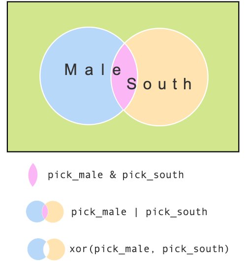

Venn diagram: different logical operations and their colors

color[pick$male]
color[pick$south]
color[pick$maleOsouth]
color[pick$maleXOsouth]

---

Other joint conditions:

# For those who are male, but not from South
pick$maleXsouth <- 
  pick$male & !pick$south
color[pick$maleXsouth]

# For those who are neither male nor from south
pick$XmaleXsouth <-
  !pick$male & !pick$south
color[pick$XmaleXsouth]

This is for the logic frenzy. Logically speaking,

NOT(NOT condition_1) # the same as
condition_1

!(! pick$male) # the same as
pick$male

---

NOT (condition_1 AND condition_2) # the same as
(NOT condition_1 OR NOT condition_2)

!(pick$male & pick$south) # the same as
!pick$male | !pick$south

---

NOT (condition_1 OR condition_2) # the same as
(NOT condition_1 AND NOT condition_2)

!(pick$male | pick$south) # the same as
!pick$male & !pick$south

& and | can be stretched to test more than 2 conditions.

# test if all three conditions are met
pick_condition1 & pick_condition2 & pick_condition3

# test if any of the three conditions is met
pick_condition1 | pick_condition2 | pick_condition3

4.6.3.1 any() and all()

In Pick and Which section, we learn that [pick] is a conditional retrieval that when attached to a vector is to answer a question like:

• For those who(se) … (defined by pick), what are their … values (defined by the object [pick] attached to)

For those who are male, what are their ages.

age[pick$male]

Sometimes, your question is like

• Is there any male?

• Are all of them male?

pick$male carries all the information needed to answer the question–no conditional retrieval needed.

The way to answer those two question is to use any() and all()

any(pick$male)
all(pick$male)

• any(): any of those are …?

• all(): all of those are …?

When NA is in your pick, be aware:

pick2 <- c(T, T, NA)
any(pick2)
all(pick2)

Exercise 4.14 Get fraud$data from exercise 2 in Exercise section. The following questions exclude any NA.

1. Convert 通報日期 to a date class. Is there any NA after conversion?

2. How many LINE accounts were reported as a fraud after 2018 (i.e. starting from 2019-01-01)?

3. How many LINE accounts were reported as a fraud between year 2019 and 2020?

4.6.4 Common situations on different vectors

Character vector

multiple hobbies

hobby = c(
  'sport, reading, movie',
  'sport',
  'movie, sport, reading',
  'movie, Reading',
  'sport')

• Who likes to read?

• Count for each hobby.

---

• to detect: who likes to read?

# any one likes to read
stringr::str_detect(hobby, "reading") # 4th is FALSE
stringr::str_detect(hobby, coll("reading", ignore_case = T)) # 4th is TRUE

Exercise 4.15 In johnDoe data,

1. Find the subsample of those whose report unit (通報機關名稱) has the term “海巡隊” (i.e. detect “海巡隊”) in its name.

2. How many different different 海巡隊 are there? Each reported how many dead bodies.

---

• to split: count for each hobby

# Count for each hobby
table(hobby)

unlisted_hobbies <- {
  hobby |> 
    stringr::str_split(", ") -> list_hobbies
  
  unlist(list_hobbies)
}
table(unlisted_hobbies)

glue ymd

df_dates =
  data.frame(
    year = c('2001','2001','2002','2001','2001'),
    month = c('4','10','1','1','4'),
    day = c('3','3','22','18','3')
  )

• Create a date class vector.

---

• to glue

chr_dates <- paste(df_dates$year, df_dates$month, df_dates$day)
chr_dates 
dates <- lubridate::ymd(chr_dates)
dates

Exercise 4.16 In johnDoe data set,

1. Add a column called 發現日期 to johnDoe$data which is a date class vector.

2. How many dead bodies have no discovered dates?

3. Which month has the highest report number?

Factor vector

students <-
  data.frame(
    major = c('economics','sociology','economics','sociology','sociology','finance','sociology','statistics','statistics','sociology'),
    year= c(4,1,4,3,1,4,4,2,1,3),
    credits= c(16,13,10,21,17,12,21,15,20,17)
  )

Which school?

students$major 

• define a new categorical vector based on a categorical vector.

---

Pick-and-assign

school = ""

{
  # For those whose major is economics or sociology, their school is social science. 
  pick_those = students$major %in% 
    c("economics", "sociology")
  school[pick_those] = "social science"
  
  # For those whose major is statistics or finance, their school is business
  pick_those = students$major %in% 
    c("statistics", "finance")
  school[pick_those] = "business"
}

school

---

factor-relevels

school = factor(students$major)

{
  levels(school) <- 
    c("social science","business","social science","business")
  
  school
}

school

Exercise 4.17 In johnDoe data set,

1. create a factor column called 發現季節 with levels, “spring”, “summer”, “fall” and “winter. They cover months 3-5 (for spring), 6-8 (for summer), 9-11 (for fall), and 12-2 (for winter)

2. In each season, how many dead bodies were discovered?

Workload?

students$credits

• credits: <= 12 (light), 13-20 (normal), 20+ (heavy)

---

• divide numeric vector into groups

## step 1. create cut points vector (each point is maximal value of a group)
maximalValues <- c(0, 12, 20, 30) # throw in a lowest value (0)

• light: maximal value is 12 normal: maximal value is 20 heavy: maximal value is some large number 50

## step 2: cut students$credits with maximalValues cut points
cut(
  students$credits, 
  maximalValues) -> students$load

## step 3(optional): using regroup skill to rename levels
levels(students$load) <- c("light", "normal", "heavy")

cut points c(0, 12, 20, 30)

If you want to include the lowest cut point (i.e. 0):

cut(
  students$credits, 
  maximalValues,
  include.lowest = TRUE
  ) -> students$load
levels(students$load)

4.7 Summarise one vector

class check, table and the basics

dates <- c('2016-11-15','NA','NA','1997-05-07','1995-08-25','2002-09-20','NA','NA','NA','1995-07-16', '2011-06-22')
grades <- c(29,53,26,27,55,69,NA,NA,63,NA,56)
genders <- c('Male','Female','Male','Male','Female','Female',NA,'Male','Male','Female','Female')
majors <- c('economics','economics',NA,'economics','economics','economics','economics','statistics','law','economics','law')

• Does it have the right class? Right class facilitates your work later.

dates |> class()
dates |> lubridate::ymd() -> dates
dates |> class()

Social scientists summarise data features one by one as their starting analysis step frequently. The summary is usually about:

• Is there NAs? If yes, how many?

analysis <- list()
anyNA(dates)
dates |> is.na() |> sum() -> analysis$dates$na$sum
anyNA(grades)
grades |> is.na() |> sum() -> analysis$grades$na$sum

If the feature is a numeric type:

• What is the range of the feature?

• What is its mean and median?

dates |> range()
dates |> range(na.rm=T) -> analysis$dates$range
grades |> range(na.rm=T) -> analysis$grades$range
grades |> median(na.rm=T) -> analysis$grades$mdian
grades |> mean(na.rm=T) -> analysis$grades$mean

If the feature is a factor:

• What are its possible levels? (levels, unique, table)

• How many observations in each level? (table)

• How many types? unique()

• Count in each type: table()

genders |> class()
genders |> factor() -> genders

genders |> levels() # only works for factor
genders |> unique() # returns a vector, data frame or array like x but with duplicate elements/rows removed.

Duplicated inputs:

dataSet0 <- 
  data.frame(
    dates = c('2016-11-15','1997-05-07','NA','NA','1997-05-07','1995-08-25','2002-09-20','NA','NA','NA','1995-07-16', '2011-06-22', '2016-11-15'),
    grades = c(29,27, 53,26,27,55,69,NA,NA,63,NA,56, 29),
    genders = c('Male','Male', 'Female','Male','Male','Female','Female',NA,'Male','Male','Female','Female','Male'),
    majors = c('economics','economics', 'economics',NA,'economics','economics','economics','economics','statistics','law','economics','law','economics')
)

There are duplicated records. Where are they?

View(dataSet0)
whichIsDuplicated <- which(duplicated(dataSet0))
dataSet0[whichIsDuplicated, ]

We can use unique() to clear up duplicated records:

dataSet0 <- unique(dataSet0)
dataSet0 |> duplicated() |> which()
View(dataSet0)

# na is removed before table summarisation
genders |> table()
# preliminary summary should include NA summary
genders |> table(useNA = "always") -> analysis$genders$table
analysis$genders$table

Summarise genders: There are length(genders) observations. Among them, 5 are female and 5 are male. One person has missing gender value (see analysis$genders$table).

Exercise 4.18 Summarise majors.

Exercise 4.19 Obtain wdi object from exercise 5 of the Exercise section. The following questions focus only on year 2000 (which means all the following questions implicitly start with the expression, for those from year 2000.)

1. How many observations are there?

2. The followings are iso2c values that represent a region but not a country. Take a subsample that excludes those region (i.e. a subsample that consists of countries),

iso2c_nonCountry <- c('ZH','ZI','1A','S3','B8','V2','Z4','4E','T4','XC','Z7','7E','T7','EU','F1','XE','XD','XF','ZT','XH','XI','XG','V3','ZJ','XJ','T2','XL','XO','XM','XN','ZQ','XQ','T3','XP','XU','XY','OE','S4','S2','V4','V1','S1','8S','T5','ZG','ZF','T6','XT','1W')

The following questions focus on the subsample.

3. How many countries are there?

4. Regarding Energy use (kg of oil equivalent per capita). Complete the following summary:

For Energy use (kg of oil equivalent per capita), there are … observations with … missing values. Excluding missing values, the range of energy use is between … and … kg/per capita of oil equivalent with median usage of … and mean usage of … .

The wdi$data’s feature meanings (other than iso2c, year, and country) can be found at:

browseURL(wdi$meta)

4.8 Exercise

1. John Doe

Data source: https://www.moj.gov.tw/2204/2771/2773/76135/post

johnDoe <- list()
johnDoe$source[[1]] <- "https://www.moj.gov.tw/2204/2771/2773/76135/post"
johnDoe$source[[2]] <- "https://docs.google.com/spreadsheets/d/1g2AMop133lCAsmdPhsH3lA-tjiY5fkGIqXqwdknwEVk/edit?usp=sharing"
googlesheets4::read_sheet(
  johnDoe$source[[2]]
) -> johnDoe$data

2. LINE fraud

fraud <- list()
fraud$source[[1]] <- "https://data.gov.tw/dataset/78432"
fraud$source[[2]] <- "https://data.moi.gov.tw/MoiOD/System/DownloadFile.aspx?DATA=7F6BE616-8CE6-449E-8620-5F627C22AA0D"
fraud$data <- readr::read_csv(fraud$source[[2]])

3. Drug

drug <- list()
drug$source[[1]] <- 
  "https://docs.google.com/spreadsheets/d/17ID43N3zeXqCvbUrc_MbpgE6dH7BjLm8BHv8DUcpZZ4/edit?usp=sharing"
drug$data <- 
  googlesheets4::read_sheet(
    drug$source[[1]]
  )

4. Econ survey

econSurvey <- list()
econSurvey$source[[1]] <- "https://docs.google.com/spreadsheets/d/1TtpiYpq_HjAHH3MJS20mZR3hb0oXDNCr6ybqmNjFFb8/edit?usp=sharing"
econSurvey$data <- googlesheets4::read_sheet(
  econSurvey$source[[1]]
)

5. WDI

wdi <- list()
wdi$source[[1]] <- "https://databank.worldbank.org/source/world-development-indicators#"
wdi$source[[2]] <- "https://docs.google.com/spreadsheets/d/1XHxjE3DIIdvNL-kbLR_bktxiHxmk23S6lUmn89WEedM/edit?usp=sharing"
wdi$meta <- "https://docs.google.com/spreadsheets/d/1C8b-liC8Gl9Kmkexb5uq1_TUIE3lYOt4PutPlOne80g/edit?usp=sharing"
wdi$data <- googlesheets4::read_sheet(
  wdi$source[[2]]
)